% Matlab Coding for PID Controller:
%PID_controller.m%
m=3.6; % Mass of the system
k=400; % Spring constant of the system
c=100; % Damping constant of the system
%Ki=10;% Integral gain of the controller
%Ki=50;
%Ki=100;
%Ki=500;
Ki=1000;
%Ki=2000;
%Ki=4000;
% The below mentioned state space form is derived from the equation
%x2_dot=-(k/m) x1 + (1/m) u
% x1_dot = x2
% where x1 is output displacement , x2 is output velocity and u is control
% Input
% State space form :
A(1,1)=0;
A(1,2)=1;
A(2,1)=-(k/m);
A(2,2)=0;
B(1,1)=0;
B(2,1)=1/m;
%Pole-Placement function :
%zeta=0.5;
zeta=0.7;
%zeta=0.99;
wn=sqrt(k/m); %finding natural frequency in 'rad/s'
t=wn*wn; % Holding wn^2 value in variable 't'
K_dc=1/m;% DC gain
s=tf('s'); % defining the transfer function variable 's'
G=K_dc*t/(s^2+2*zeta*wn*s+t); % transfer function representation
% pzmap(G,'r'); % pole-zero map representation of the transfer function
Y=[1 2*zeta*wn t]; % Denominator of the transfer function
p=roots(Y);% Finding the roots of the transfer function and placing in variable 'p'
K=place(A,B,p); %placement of poles to reduce oscillation in undamped system
Kp=K(1);%proportional gain
Kd=K(2);%derivative gain
Comments :
It has been attached as PID_controller1.m for your reference
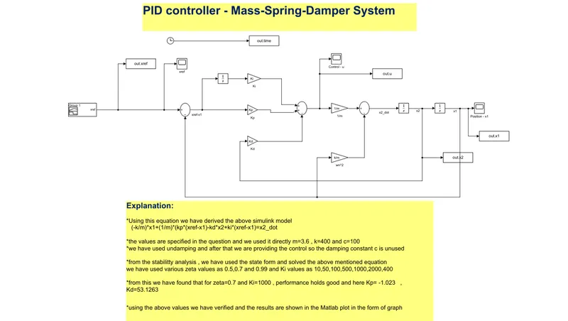
Explanation:
*Using this equation we have derived the above simulink model
(-k/m)*x1+(1/m)*(kp*(xref-x1)-kd*x2+ki*(xref-x1)=x2_dot
*the values are specified in the question and we used it directly m=3.6 , k=400 and c=100
*we have used undamping and after that we are providing the control so the damping constant c is unused
*from the stabilitty analysis , we have used the state form and solved the above mentioned equation
we have used various zeta values as 0.5,0.7 and 0.99 and Ki values as 10,50,100,500,1000,2000,400
*from this we have found that for zeta=0.7 and Ki=1000 , performance holds good and here Kp= -1.023 , Kd=53.1263
*using the above values we have verified and the results are shown in the Matlab plot in the form of graph
Comments :
It has been attached as PIDcontroller_MassSpringDamperSystem13.mdl for your reference
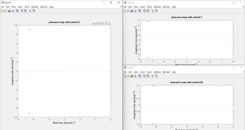
The above plot shows pole zero mapping for zeta values = 0.5,0.7,0.99
Comments :
It has been attached as mapp.m for your reference
%Matlab coding:
figure(12);
pzmap(G,'r');
title('pole-zero map with zeta=0.99');
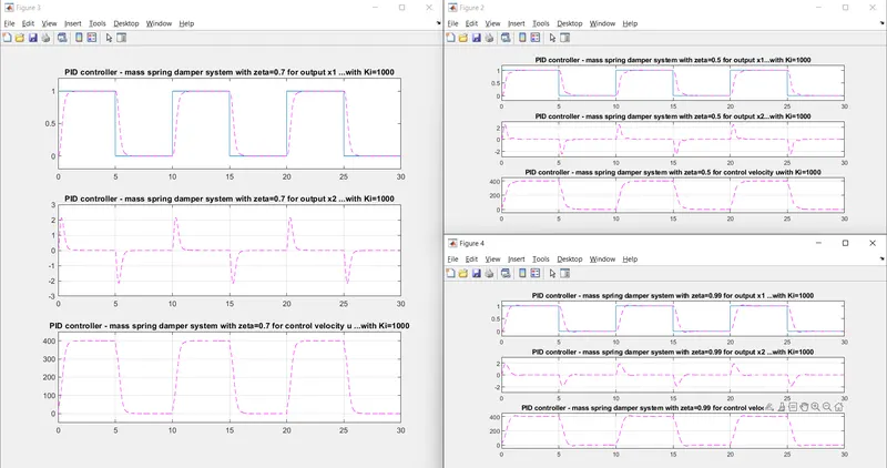
The above plot shows plots for zeta values = 0.5,0.7,0.99 with Ki=1000
Comments :
It has been attached as representation.m,representation1.m,representation2.m for your reference
%Matlab coding:
%representation.m
figure(2);
subplot(3,1,1);
plot(out.time,out.xref);grid;hold;
plot(out.time,out.x1,'m--');grid;hold;
title(['PID controller - mass spring damper system with zeta=0.5 for output x1...' ...
'with Ki=1000']);
v=axis;
v(3)=-0.2;
v(4)=1.2;
axis(v);
subplot(3,1,2);
plot(out.time,out.x2,'m--');grid;
title(['PID controller - mass spring damper system with zeta=0.5 for output x2...' ...
'with Ki=1000']);
v=axis;
v(3)=-3;
v(4)=3;
axis(v);
subplot(3,1,3);
plot(out.time,out.u,'m--');grid;
title(['PID controller - mass spring damper system with zeta=0.5 for control velocity u' ...
'with Ki=1000']);
v=axis;
v(3)=-50;
v(4)=450;
axis(v);
%representation1.m
figure(3);
subplot(3,1,1);
plot(out.time,out.xref);grid;hold;
plot(out.time,out.x1,'m--');grid;hold;
title(['PID controller - mass spring damper system with zeta=0.7 for output x1 ...' ...
'with Ki=1000']);
v=axis;
v(3)=-0.2;
v(4)=1.2;
axis(v);
subplot(3,1,2);
plot(out.time,out.x2,'m--');grid;
title(['PID controller - mass spring damper system with zeta=0.7 for output x2 ...' ...
'with Ki=1000']);
v=axis;
v(3)=-3;
v(4)=3;
axis(v);
subplot(3,1,3);
plot(out.time,out.u,'m--');grid;
title(['PID controller - mass spring damper system with zeta=0.7 for control velocity u ...' ...
'with Ki=1000']);
v=axis;
v(3)=-50;
v(4)=450;
axis(v);
%representation2.m
figure(4);
subplot(3,1,1);
plot(out.time,out.xref);grid;hold;
plot(out.time,out.x1,'m--');grid;hold;
title(['PID controller - mass spring damper system with zeta=0.99 for output x1 ...' ...
'with Ki=1000']);
v=axis;
v(3)=-0.2;
v(4)=1.2;
axis(v);
subplot(3,1,2);
plot(out.time,out.x2,'m--');grid;
title(['PID controller - mass spring damper system with zeta=0.99 for output x2 ...' ...
'with Ki=1000']);
v=axis;
v(3)=-3;
v(4)=3;
axis(v);
subplot(3,1,3);
plot(out.time,out.u,'m--');grid;
title(['PID controller - mass spring damper system with zeta=0.99 for control velocity u..' ...
'with Ki=1000']);
v=axis;
v(3)=-50;
v(4)=450;
axis(v);
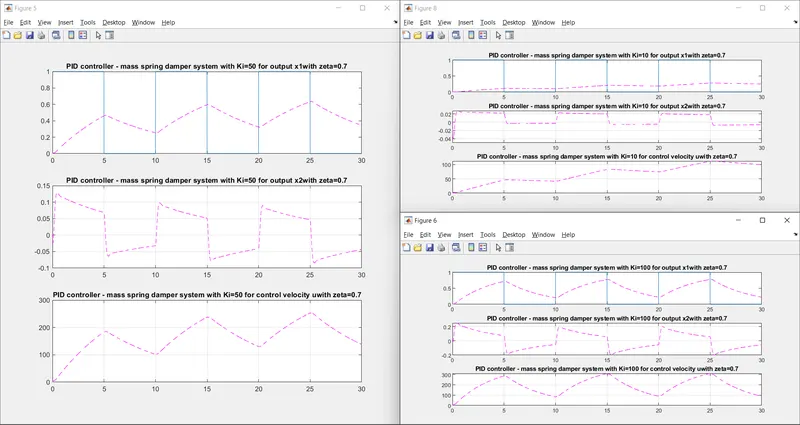
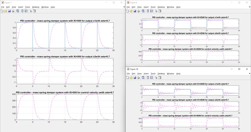
The above plot shows for zeta values = 0.7 with Ki as 10,50,100,500,1000,2000,4000
Comments :
It has been attached as intgrl.m ,intgrl1.m ,intgrl2.m ,intgrl3.m ,intgrl4.m ,intgrl5.m for your reference
%Matlab coding:
%intgrl.m
figure(5);
subplot(3,1,1);
plot(out.time,out.xref);grid;hold;
plot(out.time,out.x1,'m--');grid;hold;
title(['PID controller - mass spring damper system with Ki=50 for output x1' ...
'with zeta=0.7']);
subplot(3,1,2);
plot(out.time,out.x2,'m--');grid;
title(['PID controller - mass spring damper system with Ki=50 for output x2' ...
'with zeta=0.7']);
subplot(3,1,3);
plot(out.time,out.u,'m--');grid;
title(['PID controller - mass spring damper system with Ki=50 for control velocity u' ...
'with zeta=0.7']);
%intgrl1.m
figure(6);
subplot(3,1,1);
plot(out.time,out.xref);grid;hold;
plot(out.time,out.x1,'m--');grid;hold;
title(['PID controller - mass spring damper system with Ki=100 for output x1' ...
'with zeta=0.7']);
subplot(3,1,2);
plot(out.time,out.x2,'m--');grid;
title(['PID controller - mass spring damper system with Ki=100 for output x2' ...
'with zeta=0.7']);
subplot(3,1,3);
plot(out.time,out.u,'m--');grid;
title(['PID controller - mass spring damper system with Ki=100 for control velocity u' ...
'with zeta=0.7']);
%intgrl2.m
figure(7);
subplot(3,1,1);
plot(out.time,out.xref);grid;hold;
plot(out.time,out.x1,'m--');grid;hold;
title(['PID controller - mass spring damper system with Ki=500 for output x1' ...
'with zeta=0.7']);
subplot(3,1,2);
plot(out.time,out.x2,'m--');grid;
title(['PID controller - mass spring damper system with Ki=500 for output x2' ...
'with zeta=0.7']);
subplot(3,1,3);
plot(out.time,out.u,'m--');grid;
title(['PID controller - mass spring damper system with Ki=500 for control velocity u' ...
'with zeta=0.7']);
%intgrl3.m
figure(8);
subplot(3,1,1);
plot(out.time,out.xref);grid;hold;
plot(out.time,out.x1,'m--');grid;hold;
title(['PID controller - mass spring damper system with Ki=10 for output x1' ...
'with zeta=0.7']);
subplot(3,1,2);
plot(out.time,out.x2,'m--');grid;
title(['PID controller - mass spring damper system with Ki=10 for output x2' ...
'with zeta=0.7']);
subplot(3,1,3);
plot(out.time,out.u,'m--');grid;
title(['PID controller - mass spring damper system with Ki=10 for control velocity u' ...
'with zeta=0.7']);
%intgrl4.m
figure(9);
subplot(3,1,1);
plot(out.time,out.xref);grid;hold;
plot(out.time,out.x1,'m--');grid;hold;
title(['PID controller - mass spring damper system with Ki=2000 for output x1' ...
'with zeta=0.7']);
subplot(3,1,2);
plot(out.time,out.x2,'m--');grid;
title(['PID controller - mass spring damper system with Ki=2000 for output x2' ...
'with zeta=0.7']);
subplot(3,1,3);
plot(out.time,out.u,'m--');grid;
title(['PID controller - mass spring damper system with Ki=2000 for control velocity u' ...
'with zeta=0.7']);
%intgrl5.m
figure(10);
subplot(3,1,1);
plot(out.time,out.xref);grid;hold;
plot(out.time,out.x1,'m--');grid;hold;
title(['PID controller - mass spring damper system with Ki=4000 for output x1' ...
'with zeta=0.7']);
subplot(3,1,2);
plot(out.time,out.x2,'m--');grid;
title(['PID controller - mass spring damper system with Ki=4000 for output x2' ...
'with zeta=0.7']);
subplot(3,1,3);
plot(out.time,out.u,'m--');grid;
title(['PID controller - mass spring damper system with Ki=4000 for control velocity u' ...
'with zeta=0.7']);
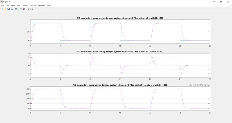
The above picture shows the best possibility result which was happened for zeta=0.7 and Ki=1000