Project - Position control of mass spring damper system
Obtain the transfer function of a mass spring damper system and use it in the model. Add a PID controller to adjust the force on mass so that its position follows a reference signal.
Take m = 3.6; %kg k = 400; %N/m c = 100; %Ns/m
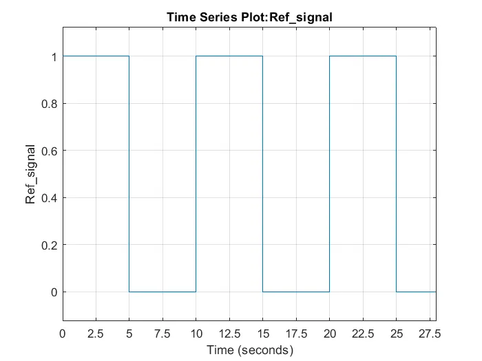
The reference signal is shown in the following figure.
Solution :
consider a simple Spring-mass-Damper system:
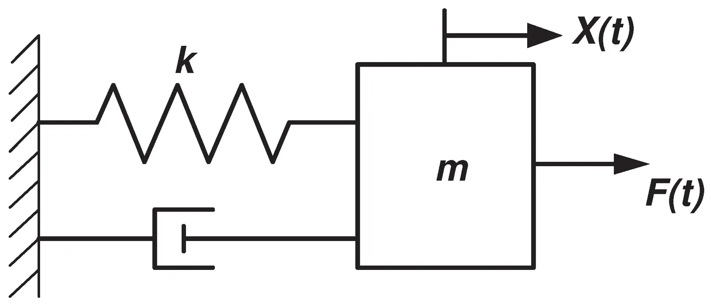
we know that the equation is as follows: in time domain
`=>f(t) = m ddotx + c dot x + kx`
this can be written in the s-domain and used to form a Transfer Function as:
`=>F(s) = (ms^2 + cs + k)X(s)`
`=>(X(s))/(F(s)) = 1/(ms^2 + cs + k)`
so we found out the Transfer Function as:
`=>(X(s))/(F(s)) = 1/(ms^2 + cs + k)`
comparing with the standard form of Second Order System TF:
`=>G(s) = (Komega_n^2)/(s^2 + 2 zeta omega_n s + omega_n^2)`
comparing the two systems(Spring-Mass-Damper and Standard Second Order System):
`=>(Komega_n^2)/(s^2 + 2 zeta omega_n s + omega_n^2) = 1/(ms^2 + cs + k)`
comparing the characteristic equation we get:
`=>s^2 + 2 zeta omega_n s + omega_n^2 = 0`
`=>ms^2 + cs + k = 0`
`=>s^2 + (c/m)s + (k/m) = 0`
comparing we can say that :
`=> omega_n = sqrt(k/m)`
`=> c/m = 2 zeta omega_n => zeta = c/(2 sqrt(mk))`
we have been provided the values of the parameters as follows:
`=>m = 3.6 "kg"`
`=>k = 400 "N/m"`
`=>c = 100 "Ns/m"`
so let us see the expected response from the system:
as we know that :
`=>zeta = c/(2 sqrt(mk))`
substituting the values we will get
`=> zeta = 100/(2 xx sqrt(3.6xx400))`
`=> zeta = 1.3176`
since `zeta>1` we expect an Overdamped Natural characteristics.
we can verify this using a test signal - step signal with amplitude=1
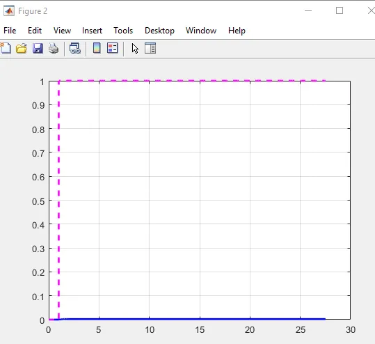
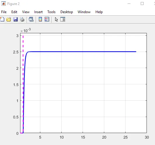
Fig: natural characterisitics of the system. We see it is very low and undamped in nature
we can predict from this behavior that the Proportional gain needed will be very high for the reference signal when we will design PID controller gains. Because naturally its amplitude only reaches to 0.0025.(see zoomed inage above).
Implementation:
since we have been asked to implement the Transfer Function of the system we will use the transfer function block for implementing the system.
we can define the parameters in the workspace using a MATLAB script and use the variables in the Simulink model.
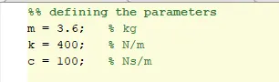
Fig: defining the variables in the script
we have to create the model in such a way that it tracks a reference signal for displacement.This means that we have to take the Output from the PID controller which will be the Forcing function in such a way that the error between the actual displacement signal and the desired referene displacement signal is minimum and it follows/tracks the refereence signal as close as possible
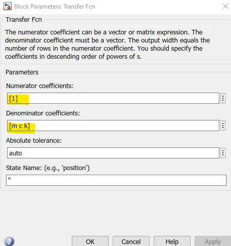
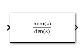
Fig: implementing the Transfer Function of the system in Transfer function block
we also have to create the reference displacement signal as provided:
Fig: reference displacement signal provided
we see that the signal provided is periodic in nature, Pulse signal with : Amplitude = 1 ,Time Period=`10s` & Pulse Width = `5/10 xx 100 = 50%` and delay of 0s
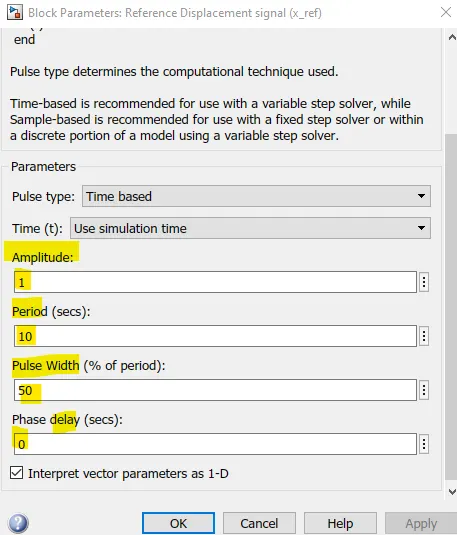
Fig: Implementing the above parameters as Pulse Generator configuration
we can implement the same reference signal as follows: using a pulse generator and defining the above parameters
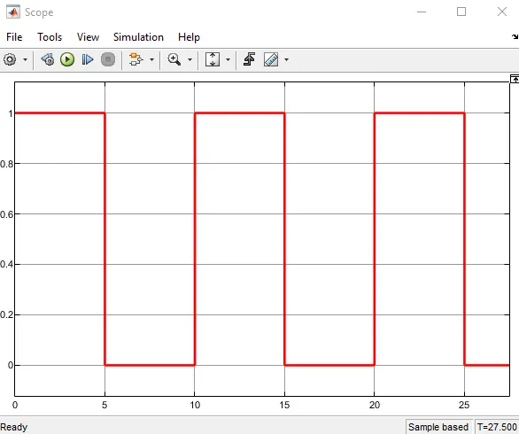
Fig: we see we implemented the reference displacement signal successfully
Simulink model:
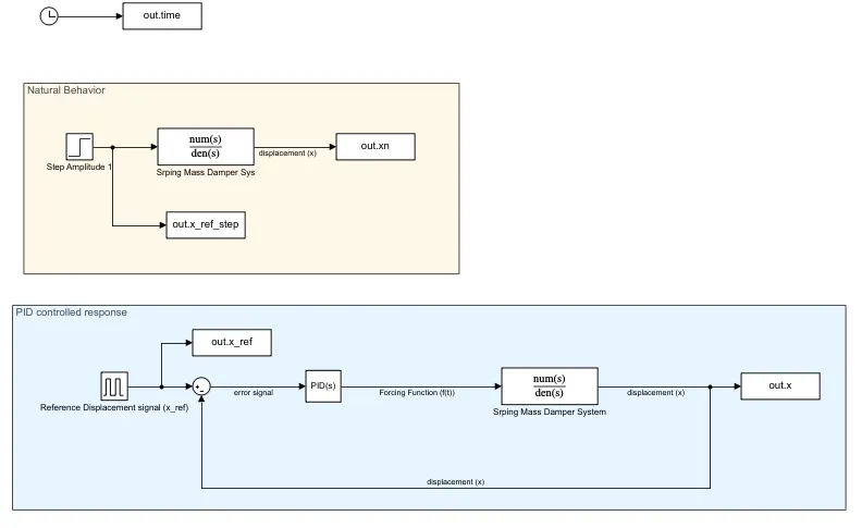
Fig: Pink-to plot and observe the open loop response. Cyan- PID tuned response
we can easily plot the responses from the simulation data in the workspace
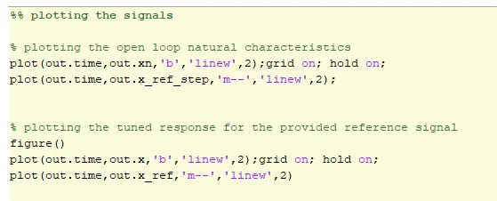
Fig: code for plotting the graphs
Response of the Closed Loop with PID controller
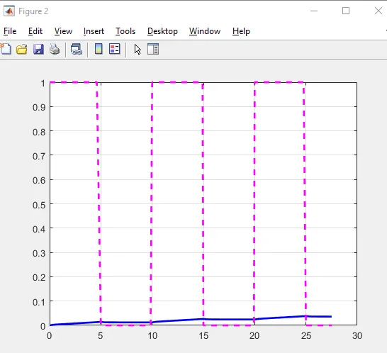
Fig: response with untuned PID with default values `=>K_p = 1, K_i=1, K_d = 0`
After tuning the controller witht the built-In tuner to get the desired response:
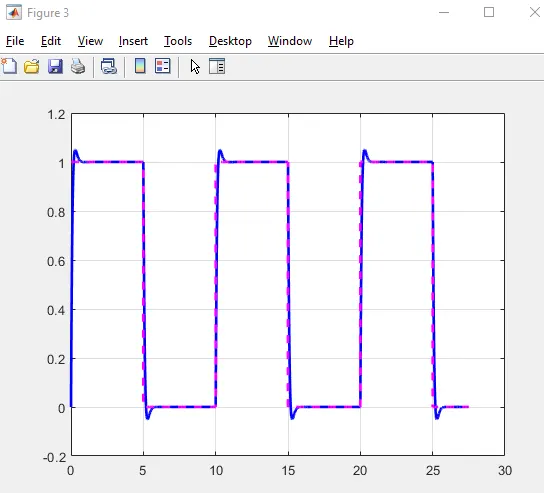
Fig: response with tuned PID with values `=>K_p = 1342, K_i=7857, K_d = 41.6, N=1516`
Response of the System: we see that the System now follows the reference displacement signal closely/ The overshoot is less than 5% and the respnse settles within 2% of final value within 0.48s and steady state error becomes 0 around 0.3sec after the abrupt pulse changes.
Note: all initial conditions were set to 0 in this case.