Challenge

Project - Position control of mass spring damper system

MMohan Jayavel24 Dec 2022

MATLAB

Question : Position control of Mass Spring Damper System - PID Controller Gains :-

Given data :-

m = 3.6; %kg

k = 400; %N/m

c = 100; %Ns/m

The reference signal figure.

Mass_Spring_Damper_System Transfer function :-

Mass :-

F=m*a=m*x_dot_dot; % m-mass F-force applied a-acceleration

Spring :-

F=k*x; % k-spring constant x-displacement

Damper :-

F=c*v=c*x_dot; % c-frictional coefficient v-velocity

MSDS :-

Input : F-force

Output : x-displacement

F-c*x_dot-k*x=m*x_dot_dot

F=m*x_dot_dot+c*x_dot+k*x

F=m*s^2*x+c*s*x+k*x

F=x*(m*s^2+c*s+k)

G(s)=x/F=1/(m*s^2+c*s+k)

PID_Controller for MSDS force adjustment :-

The above transfer function which is functioning MSDS and the force on mass has been controlled by PID of having following functioning equation

u(t)=kp*e(t)+ki*int.e(t)dt+kd*(de(t)/dt)

Model making of Mass Spring Damper System - PID Controller gains :-

Open new simulink model
Open simulink library to pick required blocks for model generation
Now, In library clock,out.simout block,step block,pulse generator block,PIDs block,gain blocks,sum,integrator blocks,transfer function blocks and scope blocks have been selected and dragged to the blank model creation.
All the blocks are connected asper control system model and using double click dialog box has been shown for parameter set.
MSDS simulink model has been modelled first and then PID Controller gain blocks are connected with MSDS block and for various speed inputs the output parameters related to Kp,Kd and Ki gains have been plotted.
After saving file, In model setting we can set required simulation parameters apply ok then run the simulation model
Now the output waveform signals of various speed values of Kp,Kd and Ki gains for given trsnsfer function response have been displayed in the form of plots by using scope block
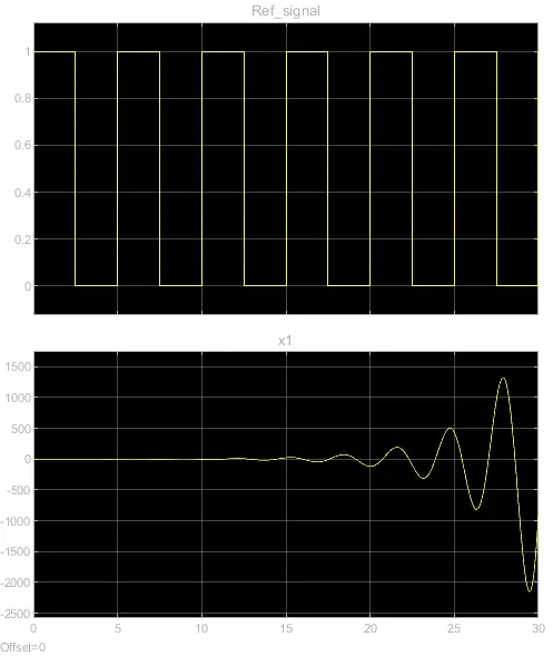
The force on mass has been gradually reduced by using Kp Kd Ki gains increased values as shown below.

MATLAB script Mass_Spring_Damper_System_PID_transferfcn.m

clc,clear all

% System parameters

m=3.6; % kg

k=400; % N/m

c=100; % Ns/m

n=[1]

d=[m c k]

G=tf(n,d)

step(G)

hold on

kp=5;

kd=25;

ki=0.5;

% Gc=pid(kp,ki,kd)

% Gcl=feedback(Gc*G,1)

% step(Gcl)

MATLAB Command window for Mass_Spring_Damper_System_PID_transferfcn :-

n =

d =

3.6000 100.0000 400.0000

G =

1
---------------------
3.6 s^2 + 100 s + 400

Continuous-time transfer function.

kp =

kd =

ki =

Gc =

Kp = 1

P-only controller.

Gcl =

1
---------------------
3.6 s^2 + 100 s + 401

Continuous-time transfer function.

>> kp

kp =

kd =

ki =

>> kp

kp =

kd =

ki =

0.5

>> kp

kp =

kd =

ki =

0.5

>> kp

kp =

kd =

ki =

MSDS_PID_Controlled_Model :-

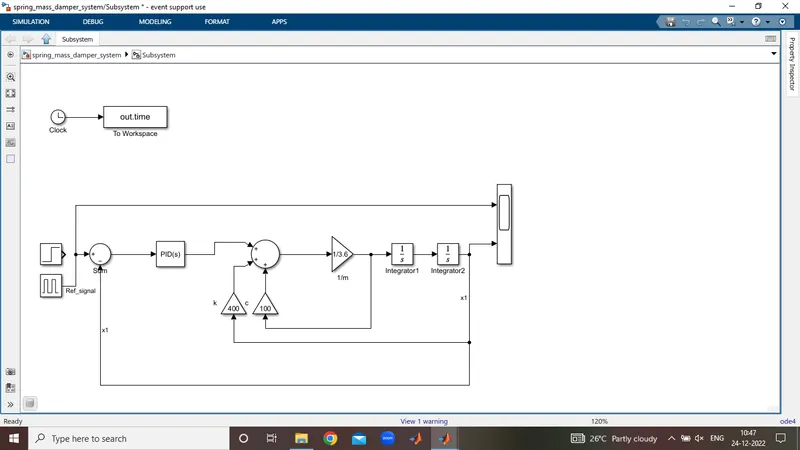
PID_Controlled_MSDS_Output

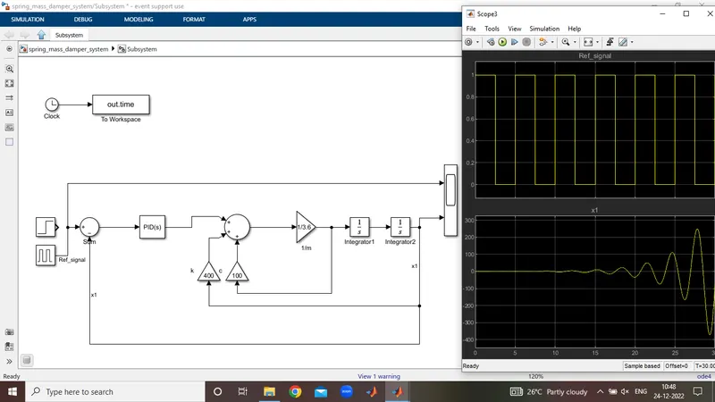
PID_Controlled_MSDS_force_adjustment_output

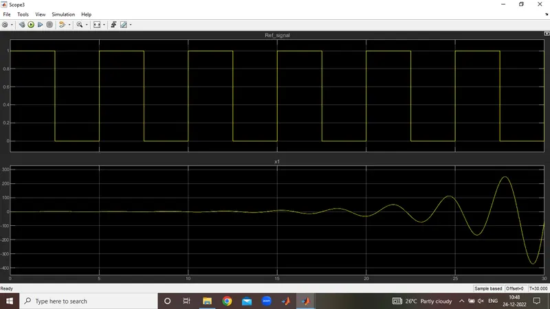
MSDS_PID_kp5kd0kp0 :-

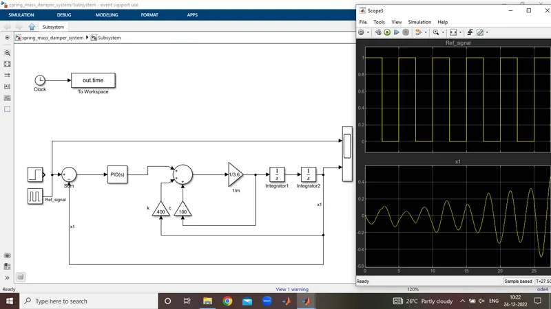
MSDS_PID_kp25kd0kp2 :-

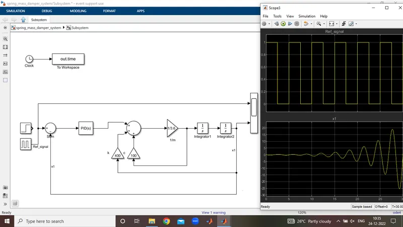
MSDS_PID_kp35kd0kp2 :-

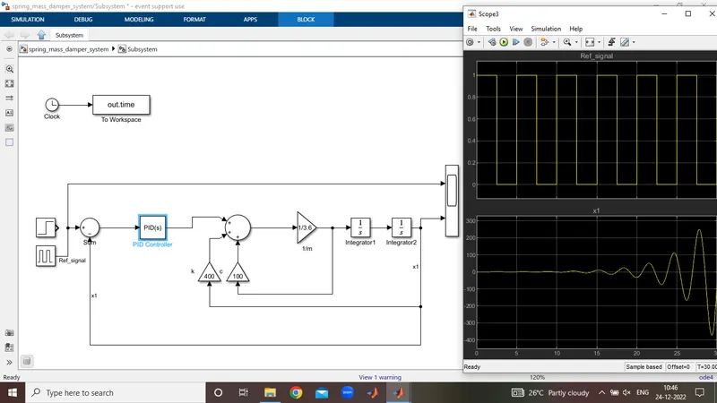
Plot_pid_smds_kp5kd15ki0.5 :-

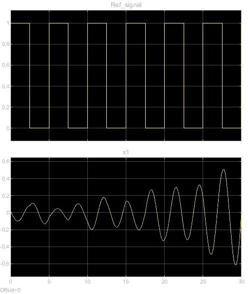
Plot_pid_smds_kp5kd25ki0.5 :-

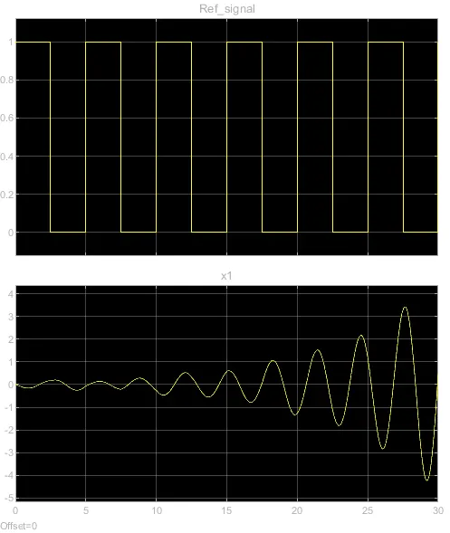
Plot_pid_smds_kp5kd35ki0.5 :-

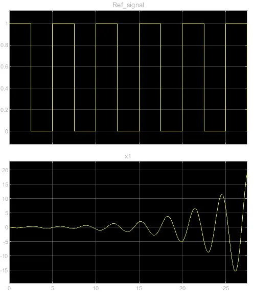
Plot_pid_smds_kp5kd15ki1 :-

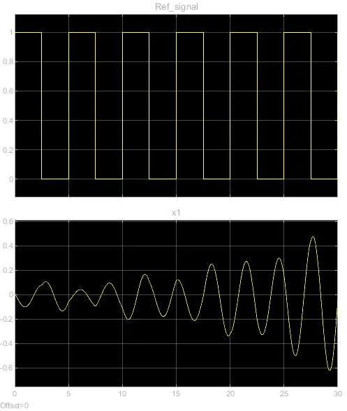
Plot_pid_smds_kp5kd25ki1 :-

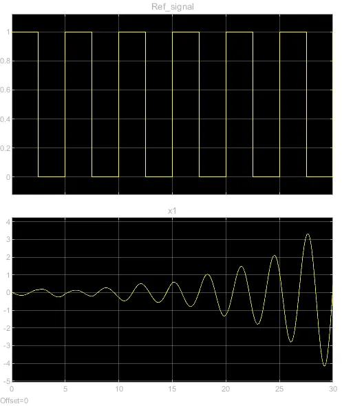
Plot_pid_smds_kp5kd35ki1 :-

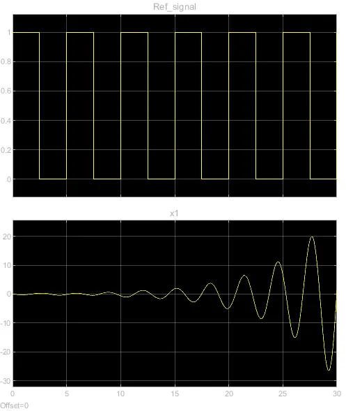
Plot_pid_smds_kp5kd25ki2 :-

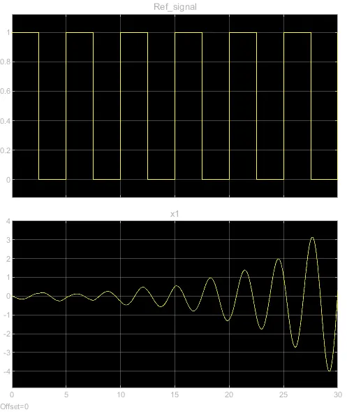
Plot_pid_smds_kp5kd35ki2 :-

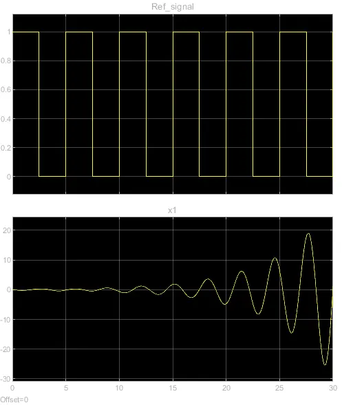
Plot_pid_smds_kp5kd50ki2 :-

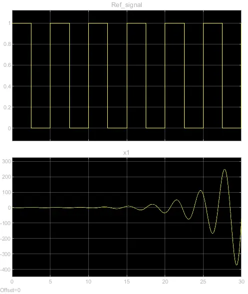
Plot_pid_smds_kp5kd60ki2 :-

Attachments :-

Simulink model for Mass_Spring_Damper_System_PID_transferfcn with Kp,Kd and Ki gains .mdl files
Waveform plots of Mass_Spring_Damper_System_PID_transferfcn screenshot .png files
Output waveform signals of gradual force on mass control values of Kp,Kd and Ki gains have been displayed in the form of plots by using scope block

Project - Position control of mass spring damper system

Ship work like this
in your own course.

Talk to a career counsellor

Ship work like thisin your own course.

Talk to a career counsellor

Ship work like this
in your own course.