QUESTION : DEVELOPMENT OF FORWARD ENERGY BASED FUEL CONSUMPTION MODEL FOR CONVENTIONAL VEHICLE
MATLAB Scripts :-
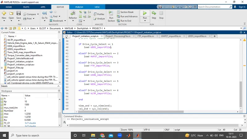
Project1_InitFile_Script of vehicle parameters and Engine parameters :-
%% Initialization File
% Initialization file for loading the variables for the Conventional vehicle simulation model
%% Vehicle Parameters
M = 1500; % Vehicle weight [kg]
Cr = 0.015; % Rolling resistance coefficient
Rw = 0.35; % Rolling radius [m]
Cd = 0.33; % Drag coefficient
Af = 2; % Frontal area [m2]
rhoa = 1.225; % Air density [kg/m3]
Vwind = 0; % Wind velocity [kmph]
g = 9.81; % Gravitational acceleration [m/s2]
theta = 0; % Slope [deg]
myu_road_tire = 1; % Coefficient of friction between tire - road interface
%% Powertrain Parameters
FDR = 3.73; % Final Drive Ratio / Diff Ratio
DiffEff = 0.99; % Differential efficiency (assumed independent of operating conditions)
NumGear = 4; % Number of gears in transmission
TransGear = [1:NumGear]; % Transmission Gears
TransRatio = [3.06, 1.62, 1, 0.7]; % Corresponding Transmission ratios
TransEff = 0.90; % Transmission efficiency (assumed independent of operating conditions)
TC_SR = [0, .5, .6, .7, .8, .87, .92, .94, .96, .97, 1]; % Torque Converter Speed Ratio (Matlab default) -> TurbSpd/PumpSpd
TC_TR = [2.232, 1.5462, 1.4058, 1.2746, 1.1528, 1.0732, 1.0192, 1, 1, 1, 1]; % Torque Converter Torque Ratio (Matlab default) -> TurbTrq/PumpTrq
TC_Cf = 1e-4 * [.72558, .66322, .63463, .59042, .51331, .4144, .29287, .22444, .12186, .04386, 0]; % Torque Converter Capacity Factor (Matlab default) -> PumpTrq/PumpSpd^2 [Nm/rpm^2]
load Vehicle_Data_Engine_data_1_9L_Saturn_95kW_importfile
load Trans_Shift_map_importfile
%% Driver Parameters
Kp = 10; % P gain for driver PI model
Ki = 1; % I gain for driver PI model
Drive_Cycle_Select = 1; % Drive cycle selection
% Drive cycle values in m/s
if Drive_Cycle_Select == 1
load UDDS_importfile;
elseif Drive_Cycle_Select == 2
load HWFET_importfile;
elseif Drive_Cycle_Select == 3
load FTP_importfile;
elseif Drive_Cycle_Select == 4
load US06_importfile;
elseif Drive_Cycle_Select == 5
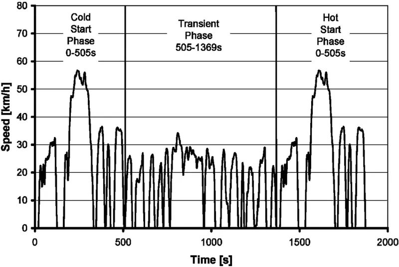
load NEDC_importfile;
elseif Drive_Cycle_Select == 6
load WLTP_importfile;
end
time_end = cyc_time(end);
vel_end = cyc_vel(end);
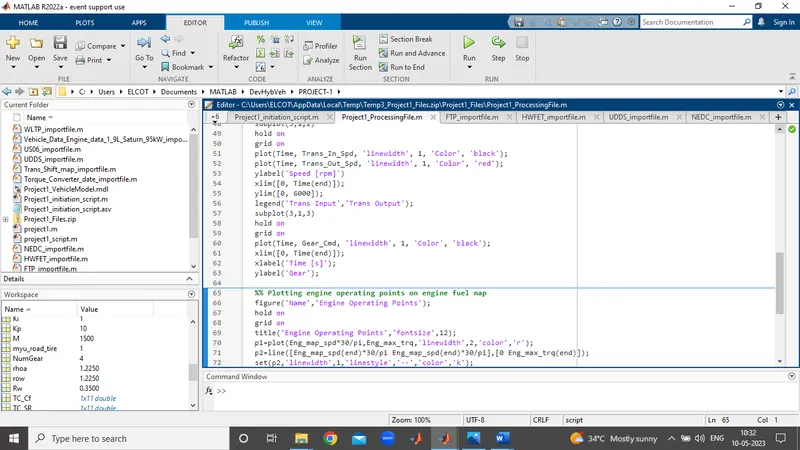
Project1_Processing file_Script for Conventional vehicle SIMULINK Model :-
% Description:
% The following file is to used with the Initialization file and Simulink
% results for post-processing of the data.
% The file is incomplete, has some examples of how the data is imported
% into a readable format, data analysis and plotting examples.
% Based on the project task, use commands in a similar format as given
% below, to analyse the data and generate required plots.
% You can change variable names if desired
%% Post-Processing File
% File for post-processing the Conventional vehicle simulation model data
%% Renaming variables
Time = out.tout;
Acc_Pdl = out.Acc_Pdl; % Accelerator pedal [%]
Brk_Pdl = out.Brk_Pdl; % Brake pedal [%]
Gear_Cmd = out.Gear_Cmd; % Transmission gear
Trans_In_Spd = out.Trans_In_Spd*30/pi; % Transmission input speed [rpm]
Trans_Out_Spd = out.Trans_Out_Spd*30/pi;% Transmission output speed [rpm]
Eng_Trq = out.Eng_Trq; % Engine brake torque [Nm]
Eng_Spd = out.Eng_Spd*30/pi; % Engine speed [rpm]
Eng_Fuel_Consump = out.Eng_Fuel_Consumption; % Engine fuel consumption [g]
Veh_Dist = out.Veh_Dist/1000; % Distance traveled by vehicle [km]
Veh_Spd = out.Veh_Spd*18/5; % Vehicle speed [kmph]
%% Data Analysis
Eng_Pwr = Eng_Spd*pi/30*Eng_Trq/1000; % Engine brake power [kW]
rho_petrol = 0.7197; % Density of petrol [kg/L]
kmpl = Veh_Dist(end)/(Eng_Fuel_Consump(end)/1000/rho_petrol); % Fuel economy [kmpl]
%% Plotting vehicle characteristics time trace
figure()
subplot(3,1,1)
hold on
grid on
plot(Time, Acc_Pdl, 'linewidth', 1, 'Color', 'black');
plot(Time, Brk_Pdl, 'linewidth', 1, 'Color', 'red');
ylabel('Pedal [%]')
xlim([0, Time(end)]);
legend('Accel','Brake');
subplot(3,1,2)
hold on
grid on
plot(Time, Trans_In_Spd, 'linewidth', 1, 'Color', 'black');
plot(Time, Trans_Out_Spd, 'linewidth', 1, 'Color', 'red');
ylabel('Speed [rpm]')
xlim([0, Time(end)]);
ylim([0, 6000]);
legend('Trans Input','Trans Output');
subplot(3,1,3)
hold on
grid on
plot(Time, Gear_Cmd, 'linewidth', 1, 'Color', 'black');
xlim([0, Time(end)]);
xlabel('Time [s]');
ylabel('Gear');
%% Plotting engine operating points on engine fuel map
figure('Name','Engine Operating Points');
hold on
grid on
title('Engine Operating Points','fontsize',12);
p1=plot(Eng_map_spd*30/pi,Eng_max_trq,'linewidth',2,'color','r');
p2=line([Eng_map_spd(end)*30/pi Eng_map_spd(end)*30/pi],[0 Eng_max_trq(end)]);
set(p2,'linewidth',1,'linestyle','--','color','k');
p3=line([Eng_map_spd(1)*30/pi Eng_map_spd(1)*30/pi],[0 Eng_max_trq(1)]);
set(p3,'linewidth',1,'linestyle','--','color','k');
[c,h] = contour(Eng_map_spd'*30/pi,Eng_map_trq,Eng_fuel_map');
clabel(c,h);
xlabel('Engine Speed [rpm]');
ylabel('Engine Torque [Nm]');
title('Engine Fuel Consumption Map [g/s]');
p4 = plot(Eng_Spd,Eng_Trq,'.','color','k');
legend([p1 p4],{'Max Curve','Operating Points'});
axis([Eng_map_spd(1)*30/pi Eng_map_spd(end)*30/pi 0 Eng_map_trq(end)]);
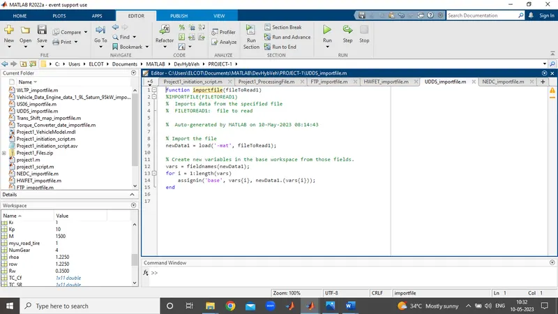
Script for computing fuel economy numbers on the urban cycle UDDS Cycle :-
function importfile(fileToRead1)
%IMPORTFILE(FILETOREAD1)
% Imports data from the specified file
% FILETOREAD1: file to read
% Auto-generated by MATLAB on 10-May-2023 08:14:43
% Import the file
newData1 = load('-mat', fileToRead1);
% Create new variables in the base workspace from those fields.
vars = fieldnames(newData1);
for i = 1:length(vars)
assignin('base', vars{i}, newData1.(vars{i}));
end
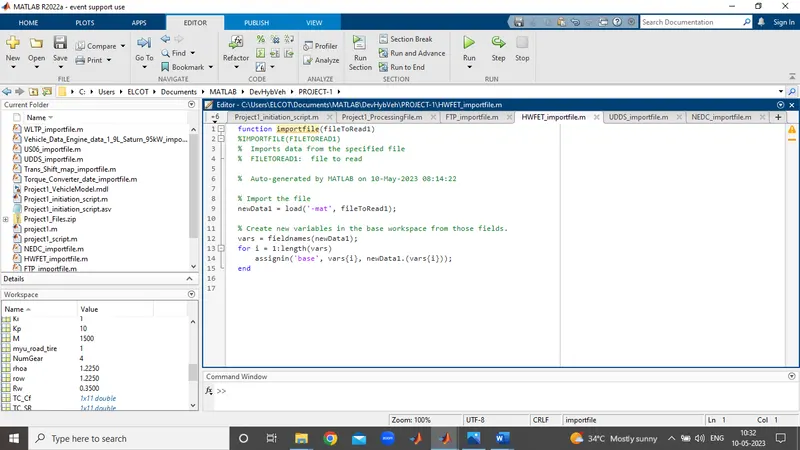
Script for computing fuel economy numbers on the highway cycle HWFET Cycle :-
function importfile(fileToRead1)
%IMPORTFILE(FILETOREAD1)
% Imports data from the specified file
% FILETOREAD1: file to read
% Auto-generated by MATLAB on 10-May-2023 08:14:22
% Import the file
newData1 = load('-mat', fileToRead1);
% Create new variables in the base workspace from those fields.
vars = fieldnames(newData1);
for i = 1:length(vars)
assignin('base', vars{i}, newData1.(vars{i}));
end
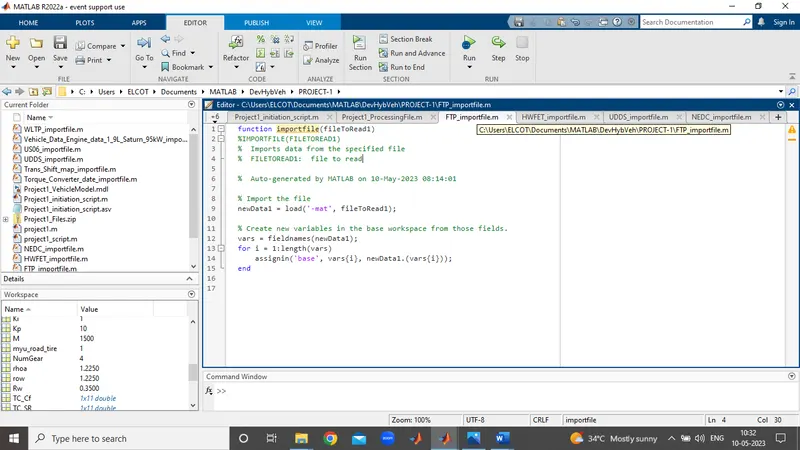
Script for computing fuel economy numbers on the FTP Cycle :-
function importfile(fileToRead1)
%IMPORTFILE(FILETOREAD1)
% Imports data from the specified file
% FILETOREAD1: file to read
% Auto-generated by MATLAB on 10-May-2023 08:14:01
% Import the file
newData1 = load('-mat', fileToRead1);
% Create new variables in the base workspace from those fields.
vars = fieldnames(newData1);
for i = 1:length(vars)
assignin('base', vars{i}, newData1.(vars{i}));
end
PROJECT REPORT ON UDDS AND HWFET DRIVE CYCLES FOR CONVENTIONAL VEHICLE WITH PERFORMANCE PLOTS :-
Fuel Economy numbers for UDDS Drive Cycle and HWFET Drive Cycles :-
'UDDS'
Fuel economy numbers =
0 0
0.0010 0
0.0020 0
0.0030 0
0.0040 0
0.0050 0
0.0060 0
0.0070 0
0.0080 0
0.0090 0
0.0100 0
0.0110 0
0.0120 0
0.0130 0
0.0140 0
0.0150 0
0.0160 0
0.0170 0
0.0180 0
0.0190 0
0.0200 0
0.0210 0.0030
0.0220 0.0059
0.0230 0.0086
0.0240 0.0115
0.0250 0.0143
0.0260 0.0169
0.0270 0.0173
0.0280 0.0181
0.0290 0.0207
0.0300 0.0217
0.0310 0.0224
0.0320 0.0225
0.0330 0.0221
0.0340 0.0215
0.0350 0.0209
0.0360 0.0204
0.0370 0.0198
0.0380 0.0170
0.0390 0.0149
0.0400 0.0149
0.0410 0.0152
0.0420 0.0155
0.0430 0.0160
0.0440 0.0171
0.0450 0.0191
0.0460 0.0211
0.0470 0.0227
0.0480 0.0229
0.0490 0.0227
0.0500 0.0226
0.0510 0.0213
0.0520 0.0190
0.0530 0.0171
0.0540 0.0158
0.0550 0.0158
0.0560 0.0177
0.0570 0.0198
0.0580 0.0216
0.0590 0.0232
0.0600 0.0242
0.0610 0.0246
0.0620 0.0249
0.0630 0.0250
0.0640 0.0246
0.0650 0.0245
0.0660 0.0247
0.0670 0.0248
0.0680 0.0247
0.0690 0.0246
0.0700 0.0246
0.0710 0.0251
0.0720 0.0256
0.0730 0.0257
0.0740 0.0254
0.0750 0.0249
0.0760 0.0250
0.0770 0.0254
0.0780 0.0260
0.0790 0.0260
0.0800 0.0257
0.0810 0.0261
0.0820 0.0267
0.0830 0.0275
0.0840 0.0286
0.0850 0.0293
0.0860 0.0298
0.0870 0.0301
0.0880 0.0304
0.0890 0.0307
0.0900 0.0307
0.0910 0.0305
0.0920 0.0304
0.0930 0.0303
0.0940 0.0304
0.0950 0.0308
0.0960 0.0304
0.0970 0.0299
0.0980 0.0295
0.0990 0.0298
0.1000 0.0303
0.1010 0.0307
0.1020 0.0309
0.1030 0.0310
0.1040 0.0309
0.1050 0.0304
0.1060 0.0298
0.1070 0.0299
0.1080 0.0302
0.1090 0.0307
'HWFET'
Fuel economy numbers =
0 0
1.0000 0
2.0000 0
3.0000 2.0000
4.0000 4.9000
5.0000 8.1000
6.0000 11.3000
7.0000 14.5000
8.0000 17.3000
9.0000 19.6000
10.0000 21.8000
11.0000 24.0000
12.0000 25.8000
13.0000 27.1000
14.0000 28.0000
15.0000 29.0000
16.0000 30.0000
17.0000 30.7000
18.0000 31.5000
19.0000 32.2000
20.0000 32.9000
21.0000 33.5000
22.0000 34.1000
23.0000 34.6000
24.0000 34.9000
25.0000 35.1000
26.0000 35.7000
27.0000 35.9000
28.0000 35.8000
29.0000 35.3000
30.0000 34.9000
31.0000 34.5000
32.0000 34.6000
33.0000 34.8000
34.0000 35.1000
35.0000 35.7000
36.0000 36.1000
37.0000 36.2000
38.0000 36.5000
39.0000 36.7000
40.0000 36.9000.....
749.0000 29.3000
750.0000 26.8000
751.0000 24.5000
752.0000 21.5000
753.0000 19.5000
754.0000 17.4000
755.0000 15.1000
756.0000 12.4000
757.0000 9.7000
758.0000 7.0000
759.0000 5.0000
760.0000 3.3000
761.0000 2.0000
762.0000 0.7000
763.0000 0
764.0000 0
765.0000 0
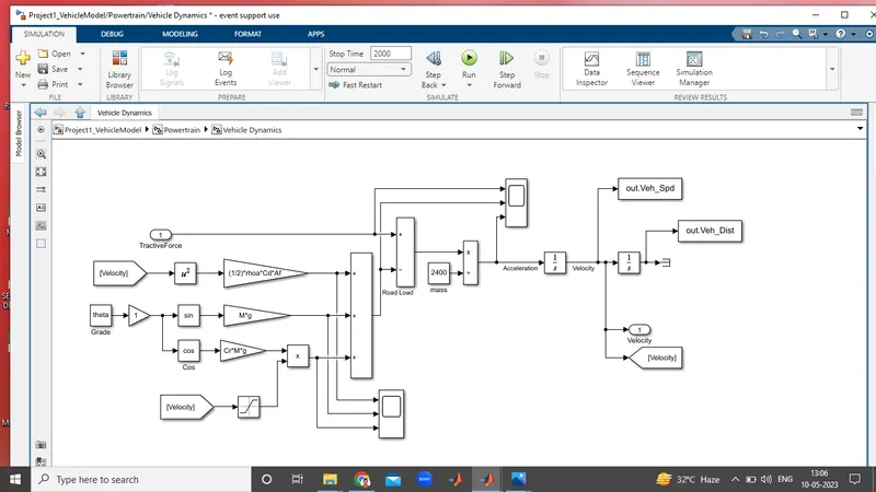
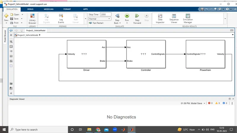
Project1_Conventional Vehicle SIMULINK Model :-
Project1_InitFile_Script :-
Project1_ProcessingFile_Script :-
DriveCycle_FTP_Script :-
DriveCycle_HWFET_Script :-
DriveCycle_UDDS_Script :-
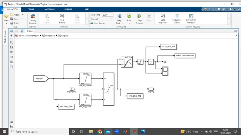
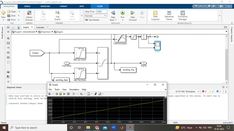
Powertrain_Engine_Model :-
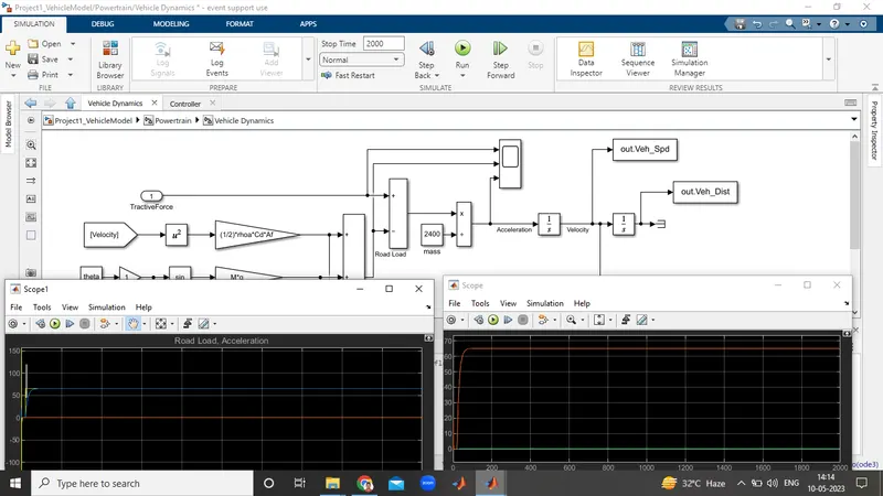
UDDS_Powertrain_Vehicle_Dynamics :-
Project1_Vehicle_Model_Run :-
Project1_Initiation_Script_Run : -
Project1_Initiation_Script Vehicle_Dynamics _Model_Run : -
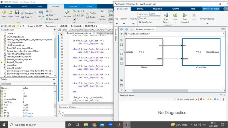
Project1_Powertrain_Run :-
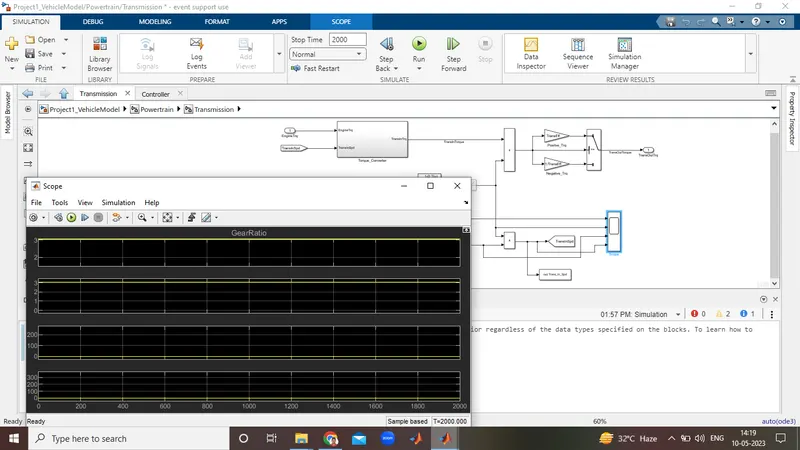
UDDS_Powertrain_Vehicle_Dynamics_Output_Plots :-
UDDS_Powertrain_Transmission_Output_Plots :-
HWFET_Powertrain_Engine_Output_Plots :-
HWFET_Powertrain_Output_Plots :-
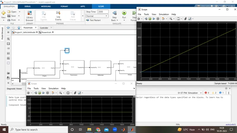
HWFET_Powertrain_Engine_Speed_Plot :-
UDDS_Road Load vs Acceleration Driver plot :-
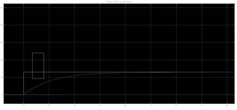
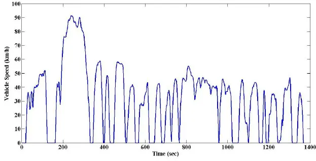
Time vs Speed UDDS Drive Cycle plot :-
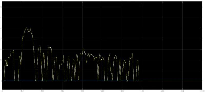
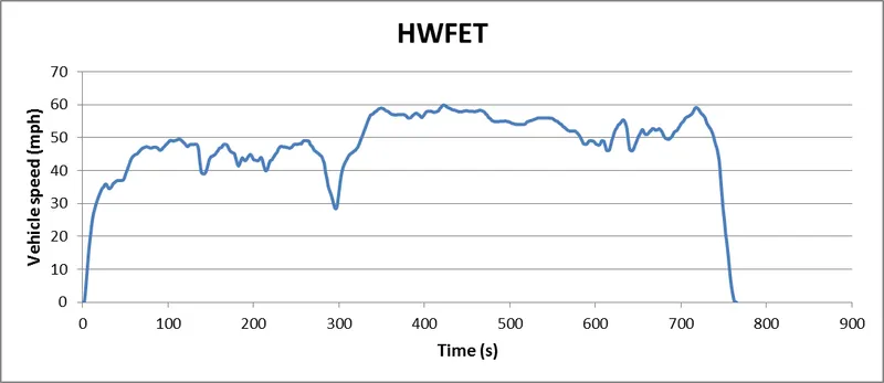
HWFET_Transmission Gear Ratio plot :-
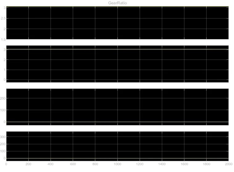
HWFET_Vehicle Dynamics Road Load vs Acceleration plot :-
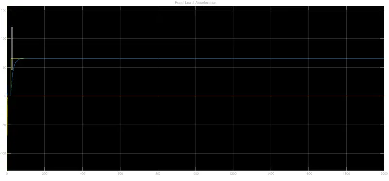
HWFET_Vehicle Dynamics Road Load vs Velocity plot :-
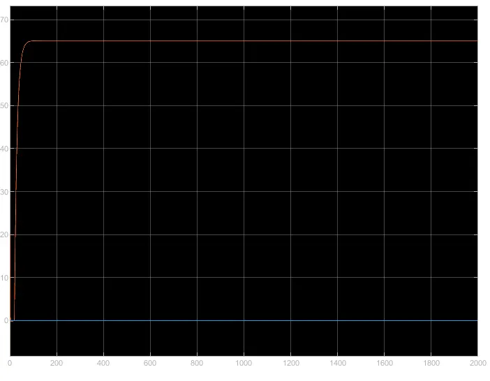
UDDS Cycle :-
HWFET Cycle :-
Combined UDDS and HWFET Cycle :-
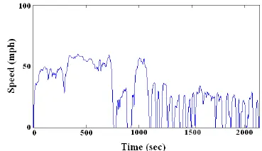
Vehicle speed vs time FTP-75 Cycle :-
ATTACHMENTS :-
- Project1 Initiation Script, Processing files, Vehicle Dynamics Model
- Transmission input output plots
- Engine torque, Engine power, fuel consumption plots
- Acceleration pedal, gear commans, vehicle actual speed subplots
- Drive cycle performance plots
-