Project - Data Handling and Interpolation

Aim: In a laboratory experiment, data of voltage and current has been recorded and the same is attached in an excel file. Read the excel file in the Matlab program and perform the interpolation in the range of -17.3:0.1:0.9. Generate the interactive plot for the interpolated data and store them in a text file.

Theory:

Interpolation

Interpolation is a method of deriving a simple function from the given discrete data set such that the function passes through the provided data points. This helps to determine the data points in between the given data ones. This method is always needed to compute the value of a function for an intermediate value of the independent function. In short, interpolation is a process of determining the unknown values that lie in between the known data points. It is mostly used to predict the unknown values for any geographical related data points such as noise level, rainfall, elevation, and so on.

A closely related problem is the approximation of a complicated function by a simple function. Suppose the formula for some given function is known, but too complicated to evaluate efficiently. A few data points from the original function can be interpolated to produce a simpler function which is still fairly close to the original. The resulting gain in simplicity may outweigh the loss from interpolation error and give better performance in calculation process.

Types of interpolation method are

1. Linear interpolation
2. Nearest neighbour interpolation or Piecewise constant interpolation
3. Polynomial interpolation
4. Spline interpolation
5. Mimetic interpolation

1. Linear interpolation

The Linear Interpolation Method applies a distinct linear polynomial between each pair of the given data points for the curves, or within the sets of three points

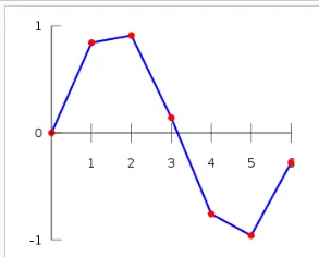
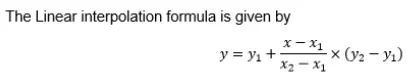
The unknown value on the data points can be found using the linear interpolation formula.

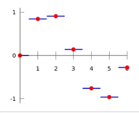
2. Nearest Nehibour Method

In this method the value of an interpolated point is inserted to the value of the most adjacent data point.Therefore the nearest neighbour method does not produce any new data points.

3. Polynomial interpolation

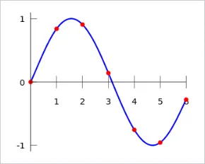
Polynomial interpolation is a generalization of linear interpolation. Note that the linear interpolant is a linear function. We now replace this interpolant with a polynomial of higher degree.

if we have n data points, there is exactly one polynomial of degree at most n−1 going through all the data points. The interpolation error is proportional to the distance between the data points to the power n. Furthermore, the interpolant is a polynomial and thus infinitely differentiable. So, we see that polynomial interpolation overcomes most of the problems of linear interpolation.

4. Spline Interpolation

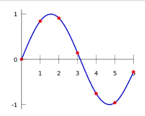
The linear interpolation uses a linear function for each of intervals [x_k,x_k+1]. Spline interpolation uses low-degree polynomials in each of the intervals, and chooses the polynomial pieces such that they fit smoothly together. The resulting function is called a spline.

For instance, the natural cubic spline is piecewise cubic and twice continuously differentiable. Furthermore, its second derivative is zero at the end points.

5. Mimetic interpolation

A key feature of mimetic interpolation is that vector calculus identites are satisfied, including Stoke's theorem and the divergence theorem. As a result, mimetic interpolation conserves line, area and volume integrals.Conservation of line integrals might be desirable when interpolating the electric field, for instance, since the line integral gives the electric potential difference at the endpoints of the integration path.Mimetic interpolation ensures that the error of estimating the line integral of an electric field is the same as the error obtained by interpolating the potential at the end points of the integration path, regardless of the length of the integration path.

Linear, bilinear and trilinear interpolation are also considered mimetic, even if it is the field values that are conserved (not the integral of the field). Apart from linear interpolation, area weighted interpolation can be considered as one of the first mimetic interpolation method to have been developed

Here, we write a program to for the given laboratory experiment, wherein we read the file & interpolate the data to finally plot all the data on two graphs. We also store the interpolated data in a text file.

Linear interpolation:

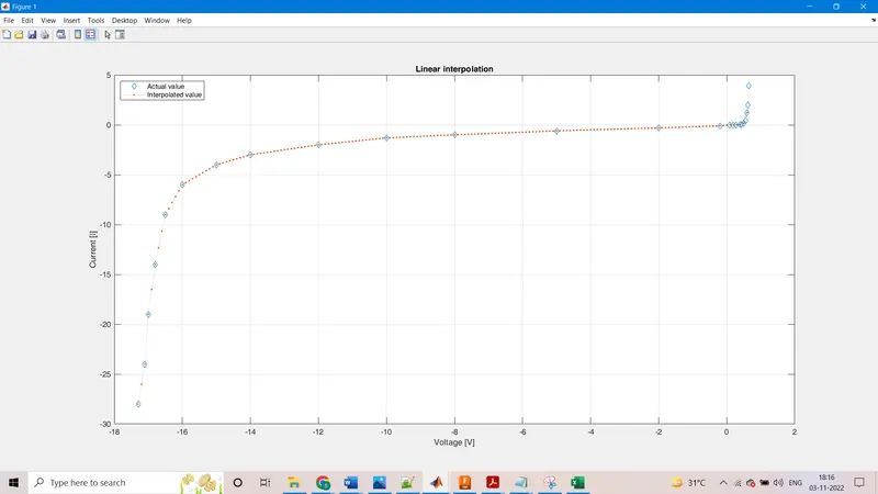
We observe that for linear interpolation many of the points pass through the curve however, the goodness of fit is visibly poor. Hence we try another interpolation

Spline Interpolation:

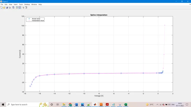
We observe that for spline interpolation, most of the points lie on the curve & this interpolation has an emmaculate goodness of fit. Hence, the spline interpolation is precise & the solution is accurate.

vi=xlsread('VI');               %reading excel file
v=vi(:,1);                      %separating voltage value
i=vi(:,2);                      %separating current value 
xq=[-17.3:0.1:0.9];             %setting interpolation range
yq1=interp1(v,i,xq);            %linear interpolated value
yq2=interp1(v,i,xq,'spline');   %spline interpolated value

figure(1)
plot(v,i,'d',xq,yq1,':.');      %ploting linear interpolation
title('Linear interpolation');
xlabel('Voltage [V]');
ylabel('Current [I]');
legend('Actual value','Interpolated value','Location','NorthWest');
grid on;

figure(2)
plot(v,i,'d',xq,yq2,'m:.');
title('Spline interpolation');  %ploting spline interpolation 
xlabel('Voltage [V]');
ylabel('Current [I]');
legend('Actual value','Interpolated value','Location','NorthWest');
grid on;

val=fopen('vi.txt','w');                 %opening text file
fprintf(val,' Voltage    Current\n');
fprintf(val,'%3.3f    %3.3f\n',xq,yq2);  %writing voltage & current value
savefig(1,'vilinear.fig');               %saving linear interpolation graph
savefig(2,'vispline.fig');               %saving spline interpolation graph
fclose(val);

The text file data is as follows: