Project
AIM :
To study and examine the BAJA All-Terrain Vehicle (ATV) model utilizing Simulink and think about various models.
Targets:-
To Prepare a specialized report making sense of the elements of the subsystems and squares utilized for setting up the model
To Explain exhaustively every one of the distinctions between every one of the five models gave
To undertand and remark on the outcomes
Introduction:
All Terrain Vehicle:
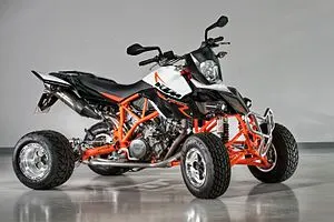
Off-road Vehicle:
An off-road vehicle (ATV) is characterized as a mechanized off-thruway vehicle intended to go on four low-pressure or non-pneumatic tires, grabbing a chair intended to be ridden by the administrator and handlebars for controlling control. ATVs are partitioned into two kinds as assigned by the producer. Type I ATVs are expected by the producer for use by a solitary administrator and no traveler. Type II ATVs are expected by the maker for use by an administrator and a traveler, and are outfitted with an assigned seating position behind the administrator.
BAJA SAE:
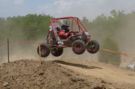
Baja SAE is a university plan series rivalry run by the Society of car engineers (SAE International). Groups of understudies from colleges all around the world plan and assemble little rough terrain vehicles. The vehicles all have motors of similar determinations. Starting around 2018 the motor has been an unmodified briggs and stratton Model 19 Vanguard motor single chamber with a removal of 305cc and power result of roughly 10 bhp (7.5 kW).
The objective in Baja SAE hustling is to configuration, construct and race rough terrain vehicles that can endure the cruelest components of harsh landscape. The vehicles utilized in Baja SAE hustling are much of the time comparable in appearance to rise carts. Before 2007, the occasions were classified "Smaller than usual Baja."
Continuously Variable Transmission(CVT):
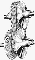
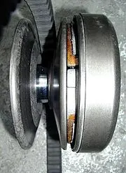
A consistently factor transmission (CVT) is anautomatic transmssion that can change flawlessly through a persistent scope of stuff proportions. This differences with different transmissions that give a predetermined number of stuff proportions in fixed advances. The adaptability of a CVT with reasonable control might permit the motor to work at a steady RPM while the vehicle moves at different paces.
Main and critical blocks used:
Generic Engine block:
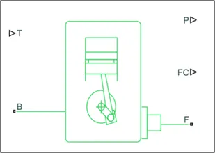
Nonexclusive Engine block:
The Generic Engine block addresses an overall gas powered motor. Motor sorts incorporate flash start and diesel. Speed-power and speed-force definitions are given. A choke actual sign information determines the standardized motor force. Discretionary unique boundaries incorporate driving rod inactivity and reaction delay. An actual sign port results motor fuel utilization rate in view of decision of fuel utilization model. Discretionary speed and redline regulators forestall motor slow down and empower journey control.
Principal ports:
B - Rotational Conserving Port :addressing the Engine Block(should be associated with rotational movement reference)
F - Rotational Conserving Port :addressing the Engine Crankshaft
T - Physical sign info port :determining the standardized motor choke level
P - Physical sign result port: detailing the momentary motor power, in W
FC - Physical sign result port: announcing the fuel utilization rate, in kg/s
Simple Gear:

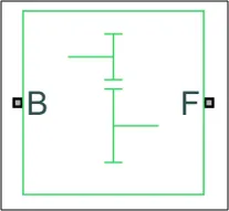
Basic Gear:
The Simple Gear block addresses a gearbox that obliges the associated driveline tomahawks of the base stuff, B, and the supporter gear, F, to corotate with a proper proportion that is determined.
The supporter base stuff proportion is
gFB=rfrB=NFNBgFB=rfrB=NFNB
Principal Ports:
B — Base: Rotational mechanical preserving port related with the base, or info, shaft.
F — Follower: Rotational mechanical rationing port related with the supporter, or result, shaft.
Variable Ratio Transmission block:
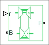
The Variable Ratio Transmission block addresses a gearbox that progressively moves movement and force between the two associated driveshaft tomahawks, base and adherent.
Disregarding the elements of transmission consistence, the driveshafts are obliged to corotate with a Variable Gear Ratio control that you control. You can pick whether the adherent pivot turns in something similar or inverse course as the base hub. In the event that they turn in a similar bearing, ωF and ωB have a similar sign. Assuming they turn in inverse bearings, ωF and ωB have inverse signs.
Transmission consistence presents inside time delay between the pivot movements. Accordingly, not at all like a stuff, a variable transmission doesn't go about as a kinematic requirement. You can likewise control force misfortune brought about by transmission and thick misfortunes.
-
Primary ports:
B - Base Pulley or Drive Pulley
F - Follower Pulley or Driven Pulley
r - Variable Transmission Ratio (Input)
Vehicle Body block:
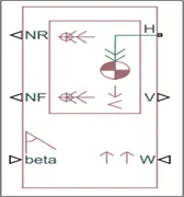
The Vehicle Body block addresses a two-hub vehicle body in longitudinal movement. The vehicle can have something similar or an alternate number of wheels on every hub. For instance, two wheels on the front hub and one wheel on the back pivot. The vehicle wheels are accepted indistinguishable in size. The vehicle can likewise have a focal point of gravity (CG) that is at or underneath the plane of movement.
The square records for weight, streamlined drag, street grade, and weight appropriation between axles because of speed increase and street profile. Alternatively incorporate pitch and suspension elements. The vehicle doesn't move upward comparative with the ground.
The square has a choice to incorporate a remotely characterized mass and a remotely characterized dormancy. The mass, dormancy, and focal point of gravity of the vehicle body can shift throughout the span of recreation in light of framework changes.
Constraints:
The Vehicle Body block allows you to show just longitudinal elements, lined up with the ground and arranged along the heading of movement. The vehicle is thought to be in pitch and ordinary balance. The square doesn't display pitch or vertical development. Accordingly, the conditions accept that the wheels never lose contact. This limitation can bring about regrettable typical powers.
Yield ports:
NR - Rear Axle Normal Force (N): actual sign result port for the back hub which is viewed as certain acting lower
NF - Front Axle Normal Force (N):physical signal result port for the front pivot which is viewed as sure acting lower
V - Longitudinal Velocity (m/s):physical yield sign of vehicle speed
Monitoring ports:
H - Horizontal Motion: monitoring port connected with the flat movement of vehicle body(tyres ought to be associated with this port)
Double shoe brake Block:
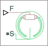
Twofold shoe brake Block:
The Double-Shoe Brake block addresses a frictional brake with two turned inflexible shoes that press against a pivoting drum to create a slowing down activity. The unbending shoes sit inside or outside the pivoting drum in an entirely gone against design. A positive activating power makes the unbending shoes press against the pivoting drum. Gooey and contact erosion between the drum and the inflexible shoe surfaces cause the pivoting drum to decelerate.
Twofold shoe brakes furnish high slowing down force with little actuator redirections in applications that incorporate engine vehicles and some large equipment. The model utilizes a straightforward definition with promptly available brake calculation and rubbing boundaries.
Constraints:
Contact points less than 45° produce less precise outcomes.
The brake utilizes the long-shoe estimation.
The brake calculation doesn't self-lock.
The model doesn't represent actuator stream utilization.
Input ports:
F - Physical sign info port related with the applied inciting force
Saving ports:
S - Rotational saving port related with the turning drum shaft
Tire(magic equation) block:
The Tire (Magic Formula) block models a tire with longitudinal conduct given by the Magic Formula, an observational condition in light of four fitting coefficients. The square can display tire elements under consistent or variable asphalt conditions.
The longitudinal course of the tire is equivalent to its bearing of movement as it rolls on asphalt. This square is an underlying part founded on the Tire street communication block.
To build the devotion of the tire model, you can indicate properties like tire consistence, latency, and moving obstruction. Nonetheless, these properties increment the intricacy of the tire model and can dial back reproduction. Consider overlooking tire consistence and latency if reproducing the model progressively or on the other hand if setting up the model for equipment in the know (HIL) reenactment.
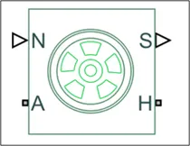
Equivalent model:
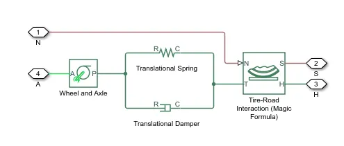
Comparable model:
The full tire model is comparable to this Simscape/Simscape Driveline part chart. It reenacts both transient and consistent state conduct and accurately addresses beginning from, and arriving at, a stop. The Translational Spring and Translational Damper are identical to the tire solidness CFx and damping bFx. The Tire-Road Interaction (Magic Formula) block models the longitudinal power Fx on the tire as a component of Fz and k′ utilizing the Magic Formula, with k′ as the autonomous slip variable.
The Wheel and Axle sweep is the wheel span rw. The Mass worth is the successful mass, Iwr2w. The tire trademark work f(k′, Fz) decides the longitudinal power Fx. Along with the driveshaft force applied to the wheel hub, Fx decides the wheel precise movement and longitudinal movement.
Without tire consistence, the Translational Spring and Translational Damper are precluded, and contact factors return to wheel factors. For this situation, the tire successfully has boundless firmness, and port P of Wheel and Axle associates straightforwardly to port T of Tire-Road Interaction (Magic Formula).
Without tire idleness, the Mass is overlooked.
Limitations:
- The Tire (Magic Formula) block assumes longitudinal motion only and includes no camber, turning, or lateral motion.
- Tire compliance implies a time lag in the tire response to the forces on it. Time lag simulation increases model fidelity but reduces simulation performance.
Normal tire boundaries:
Wizardry Formula B coefficient: 10
Wizardry Formula C coefficient: 1.9
Wizardry Formula D coefficient: 1
Wizardry Formula E coefficient: 0.97
Yield ports:
S - Tire Slip: Physical sign result port related with the overall slip between the tire and street.
Saving ports:
A - Axle: Mechanical rotational port related with the hub that the tire sits on.
H - Mechanical translational port related with the wheel center that communicates the push created by the tire to the rest of the vehicle
Different Blocks utilized:
Solver Configuration - To determine the solver boundaries prior to beginning the reenactment
Signal Builder - To enter the Brake, Throttle and CVT Ratio
Simulink to PS Converter - To change over the Simulink sign to Simscape climate
PS to Simulink Converter - To change over Simscape sign to Simulink climate
Mechanical Reference - To ensure every one of the parts are clasped to the ground
Rotational free end: The Rotational Free End block addresses a mechanical rotational port that pivots unreservedly, without force.
Scope - To show various charts
Show - To see the determined motor power
Dormancy - To address the strong inactivity
Rotational Motion Sensor - To detect the rotational movement from the motor and give yield as rpm
PS Terminator - Terminator for detached actual sign results
PS Constant - Generate steady actual sign
Rotational Free End - For mechanical part (Tire)
Custom Measure Gauge - To quantify the brake and choke input
Handle - To expand, lessening as well as the other way around of choke and brake inputs
Query Table - To embed the CVT values from the work area
Step - To increment or diminishing an information an incentive for a characterized time frame stretch
BAJA ATV MODEL WITHOUT DASHBOARD (cvtModel)
Fundamental MODEL:
Steps:
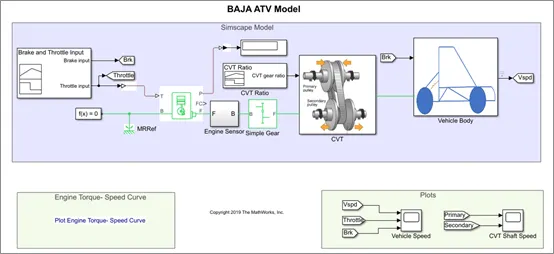
i.The choke signal is produced by signal developer block and inputted to conventional motor.
ii.The force and speed vector are inputted from the matlab work area
iii.The motor will create the result rpm which can be taken from the driving rod yield. This speed will be given to the Ideal Rotational Motion Sensor to detect the result rpm.
iv.The same result speed will be given to a straightforward stuff instrument to lessen the speed where the Gear Ratio is '4'.
v.Then the result speed from the stuff minimizer will be given to the Variable Ratio Transmission block (CVT).
vi.The CVT proportion is given to the Variable Ratio Transmission (CVT) block through Signal Builder.
vii.The speed is constrained by the variable CVT proportions and the controlled result speed is inputted to the vehicle hub.
viii.The brake signal is produced by the sign manufacturer and inputted to the vehicle body (Double Shoe Brake) for applying the brake to pivot.
ix.The power from the CVT is inputted to the hub and the vehicle speeds up as per the speed.
x.Then the Velocity is taken as result from the vehicle body for additional investigation.
Input signals:
Choke input signal:
Choke begins at 0.3 and afterward it steps to 1 at the twentieth second
Brake input signal:
The brake input stays zero through the entire reproduction
Input signals:
Throttle input signal:
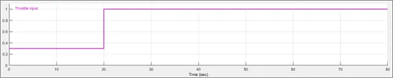
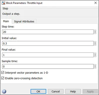
Throttle starts at 0.3 and then it steps to 1 at the 20th second
Brake input signal:

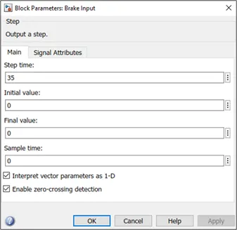
The brake input remains zero through the whole simulation
Torque and speed Matlab workspace input:
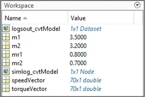
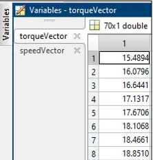
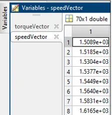
Cvt ratio input:
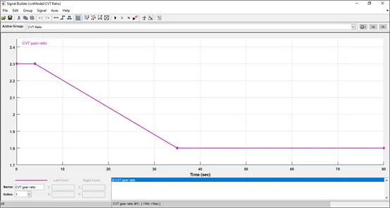
Cvt ratio starts at 2.3 ,then 5 sec it gradually reduces until it reaches 1.8 at 35th second and it remains so till the end of the simulation
Motor SENSOR SUB-BLOCK:
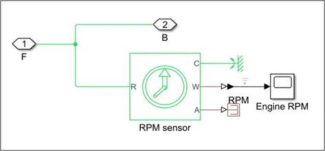
This subblock measure motor rotational speed as it takes the result of the motor as its feedback and results motor Rpm
CVT SUBBLOCK:
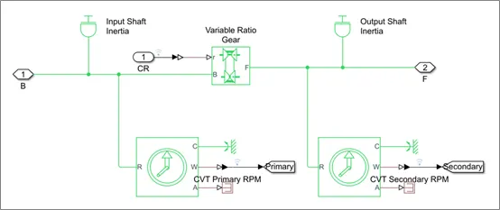
The cvt subblock gives the info and the result shafts of the cvt with latency, and measures the information shaft rpm and the result shaft rpm
Vehicle body subblock:
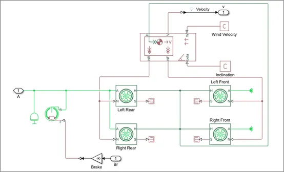
The model shows that the vehicle is back tire drive as the result from the gearbox is inputted to the back pivot, then an inactivity is added to reproduce hub latency, then the shoe brake s saving port is associated with the hub, and afterward a similar hub interfaces the two back tires while the front tires is allowed to turn on a rotational free end. Everything the tires H center point port is associated together and afterward associated with the vehicle H port, Also the back tires N port is associated together and afterward associated with the vehicle body Nr yield ports, while the front are associated with the Nf vehicle body yield ports, the vehicle body takes the street tendency and wind speed from actual constants.
Results:
Torque speed plot:
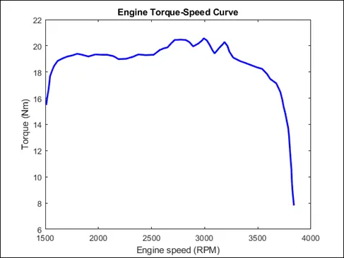
The force and speed are inputted from the matlab work area window to the nonexclusive motor square to appropriately produce the result RPM. This plot conduct is conventional to all ICE.
Engine speed plot:
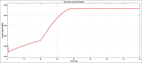
The motor rpm created by the choke, speed and force inputs. It is plainly clear the way in which the progression expansion in choke at twentieth second brought about an expansion in the motor upheavals from 2,250 to 3,800 RPM
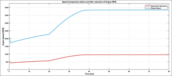
Here we can see that the motor speed is decreased by the Gear Ratio '4'.
Most extreme RPM (Before Reducing) = 3833 rpm was diminished to 958.25 rpm which can be checked by partitioning the 3833 by the stuff decrease proportion 4
CVt speed reduction plot:
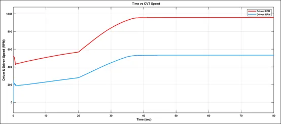
The motor decreased speed is constrained by different CVT Ratios. For check the most extreme RPM is determined at 1.8 stuff proportion which is material from the 35th second.
Most extreme RPM (Before Reducing) = 958.25 rpm
CVT Ratio = 1:1.8
GearRatio=DrivenDriverGearRatio=DrivenDriver
11.8=Driven958.2511.8=Driven958.25
Driven=958.251.8Driven=958.251.8
Driven=532.36RPMDriven=532.36RPM
The diminished most extreme rpm is 532.36 rpm which can be checked from the plot.
Speed versus choke plot:
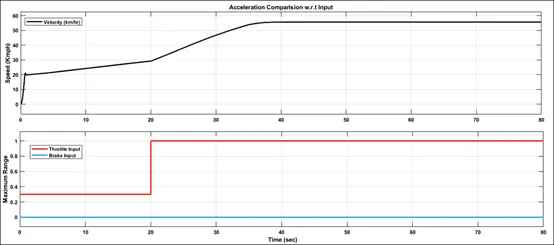
From the chart we can construe that the brake isn't applied during the drive cycle and the Throttle is consistent (0.3) till 20 sec and being expanded from 0.3 to 1 from 20 sec where it stays steady all through. With expansion in choke the vehicle speed expanded from 30 to 55 kmph.
.
BAJA ATV model - Data Extraction(cvtModel_data)
Fundamental model
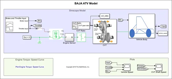
Steps:
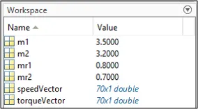
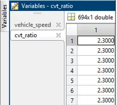
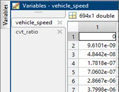
The model work process is same as the course of 'BAJA ATV model without Dashboard'. The little expansion is here the CVT Ratio and Vehicle Speed information are extricated utilizing 'To Workspace' block.
Results:
he outcomes are same as 'BAJA ATV model without Dashboard' yet an extra result is the CVT Ratio and Vehicle Velocity to the Workspace.
Before to workspace block:
After to workspace block:
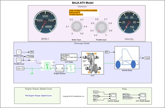
BAJA ATV MODEL WITH DASHBOARD(cvtModel_dashboard):
Main Model:
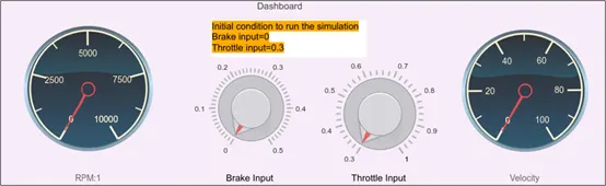
Dashboard:
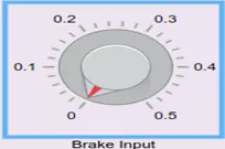
User controls:
Steps:
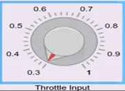
The model work process is same as the course of 'BAJA ATV model without Dashboard' yet the choke and brake inputs are constrained by the client with handles.
Results:
Engine speed plot:
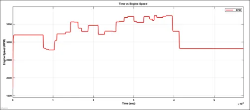
HHere the motor speed is produced by the sources of info like choke, break, force and speed vectors. The runtime isn't characterized so the Throttle and Break are constrained by the client. The move forward is choke and step down is brake input.
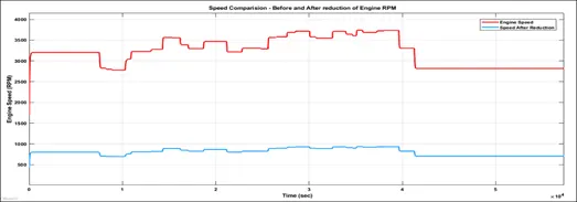
The motor speed is decreased by an element of 4 at any second in the drive cycle as it is obvious by the bend.
CVT speed reduction plot:
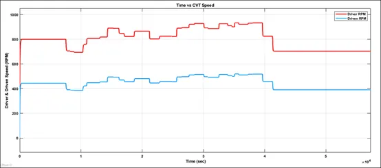
The Cvt gear decrease plot shows that at consistent the decrease proportion of 1.8 is relevant at these huge time period and it very well may be checked by taking 689 steady RPM and separating it by 1.8=383 RPM which confirms the plot
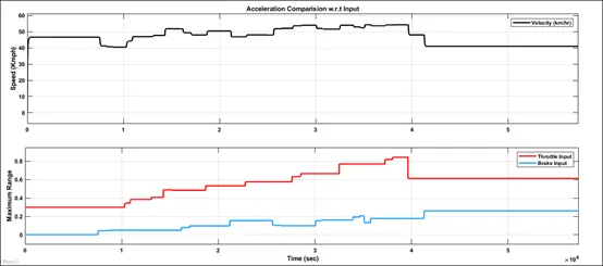
From the chart we can surmise that the vehicle is speeding up while choke is applied (Step Up) and decelerated while break is applied (Step Down). The consistent speed regions address no progressions in choke or slowing down.
BAJA ATV model - Mapped Lookup Table without Dashboard(cvtModel_mapped):
Principal model:
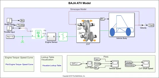
Steps:
The model work process is same as the course of 'BAJA ATV model without Dashboard' aside from that it utilized rather than Signal Builder Blocks for Brake and Throttle Input Step input blocks are utilized. At 35 sec the brake info will make a stride of significant worth '0' and at 20 sec choke information will increments from 0.3-1 then, at that point, stays steady all through.
CVT SUBBLOCK:
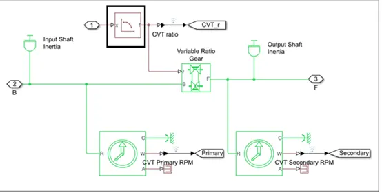
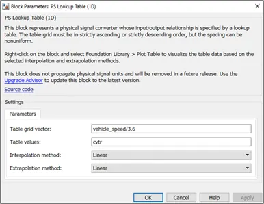
Query Table:
A query table is a variety of information that guides input values to yield values, accordingly approximating a numerical capacity. Given a bunch of information esteems, a query activity recovers the relating yield values from the table. On the off chance that the query table doesn't expressly characterize the information values, Simulink can gauge a result esteem utilizing interjection, extrapolation, or adjusting, where:
Results:
Cvt ratio plot:
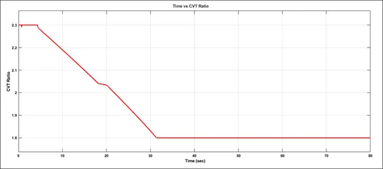
Whenever we look at the above plot, the proportion shifts from 2.3 - 1.8 inside period of time of 80 sec which is same as the past BAJA ATV Models. What's more, from 32 sec it's consistent proportion of '1.8' contrasted with 35 sec in the primary model. Likewise the decrease from 2.3 proportion to 1.8 isn't entirely direct as in the principal model.
CVT proportion versus vehicle speed:
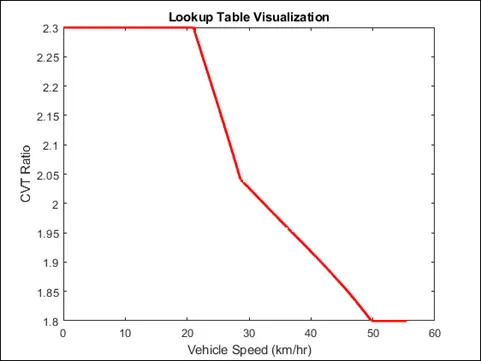
CVT proportion versus vehicle speed:
0 to 20 km/hr, the CVT proportion is consistent at 2.3
20 to 30 km/hr, the CVT proportion drops down to 2.03
30 to 50 km/hr, the CVT proportion drops down to 1.8
50 km/hr onwards, the CVT proportion is steady at 1.8
Motor speed:
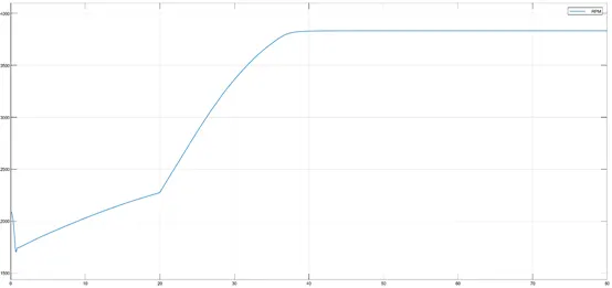
A similar diagram is displayed in the main model
CVT Shaft Speed:
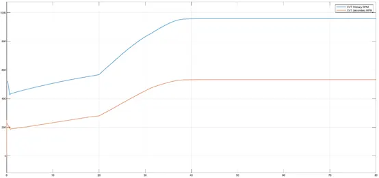
The output shaft speed follows the cvt ratio discussed before.
Speed vs. throttle plot:
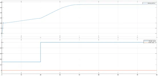
The result shaft speed follows the cvt proportion examined previously.
BAJA ATV model – Mapped Lookup Table with Dashboard(cvtModel_dashboard_mapped):
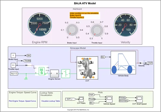
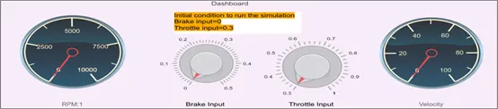
Dashboard (simulation off):
Dashboard (simulation on):
User controls:
Steps:
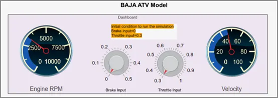
The model work process is same as the course of 'BAJA ATV model - planned query table without Dashboard' yet the Throttle and Brake inputs are constrained by the client with the Knob followed by the vehicle speed is given as criticism to the CVT Ratio query table.
CVT ratio plot:
I
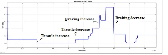
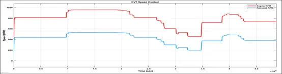
In this BAJA ATV Model, the Engine is pre-set to run at 3300 rpm with the choke worth of '0.3'. Also, the speed at 45 KMPH. The CVT Ratio for least and most extreme speed of the motor was pre-characterized as 2.3 and 1.8 individually. Whenever the reenactment is begun the underlying choke esteem 0.3 is accomplished so the CVT Ratio is close by to 1.85. At the point when the choke is being expanded the CVT Ratio move towards 1.8 where the state is most extreme motor speed. At the same time when the choke is being diminished the CVT proportion will move towards 1.85. While the slowing down is applied the CVT Ratio increments so it can accomplish the closest condition of 2.3 (Minimum Engine Speed). While slowing down is diminished the CVT Ratio move towards 1.85 which is the essential choke input 0.3 or then again assuming some other choke esteem is applied it would arrive at that CVT Ratio state.
Motor speed plot:
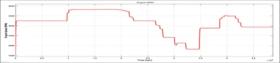
From the diagram we can deduce that the vehicle was first running at least rpm of 3300 rpm and afterward choke is applied (move forward) then, at that point, slowing down (venture down) then, at that point, brake is delivered so motor rpm is expanded then slowing down is applied.
Engine speed plot:
Cvt speed reduction plot:
Speed vs. throttle plot:
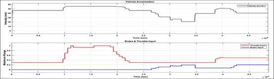
From the plot we can induce that when choke is applied the vehicle speed increments and when brake is applied vehicle speed diminishes all the while.