Week 4.1 - Genetic Algorithm

OBJECTIVE : To optimise the stalagmite function and find the global maxima of the function by using MATLAB.

Genetic Algorithm :

Hereditary Algorithm (GA) is a part of field of study called developmental comutation. It depends on development hypothesis by Darwin. GA is utilized to streamline a given capacity to track down its most extreme or least worth. The essential parts of a GA are

1. Wellness work : It is the capacity that GA is attempting to advance.

2. A populace of chromosome : It is the mathematical qualities that address every one of the answers for the capacity. The determination administrator picks a portion of the chromosomes (with substitution) for multiplication in view of likelihood dispersion. fitter the chromosome more probable it is to be chosen.

3. Get over : This administrator trades in irregular an aftereffect of two of the picked chromosomes to make two offspring. Normally every chromosome is changed over into double code and afterward get over is done from one parent chromosome into another.

4. Change : Mutation administrator haphazardly flips individual pieces in the new chromosomes.

The GA sentence structure in Matlab is given by :

x = ga(fun,nvars,A,B.Aeq.Beq,LB,UB.nonlcon,intcon,options)

Where,

fun = objective function

nvars = number of variables

A and B = subject to linear inequalities of the form A*x <=B

Aeq and Beq = subject to linear equalities of the form A*x = B

LB = lower bound

UB = upper bound

nonlcon = non linear inequalities

intcon = integer constrained

options = helps to add contraint tolerance by increasing the population size

Some advantages of genetic algorithms this method are the following:

1) They usually perform better than traditional feature selection techniques.

2) Genetic algorithms can manage data sets with many features.

3) They don't need specific knowledge about the problem under study.

4) These algorithms can be easily paralelized in computer clusters.

Working of Genetic Algorithm:

The accompanying diagram sums up how the hereditary calculation functions:

1) The calculation starts by making an irregular introductory population.The calculation then makes a succession of new populaces.

2) At each progression, the calculation involves the people in the ongoing age to make the following populace.

To make the new populace, the calculation plays out the accompanying advances:

a) Scores every individual from the ongoing populace by processing its wellness esteem. These qualities are known as the crude wellness scores.

b) Scales the crude wellness scores to change over them into a more usable scope of values. These scaled qualities are called assumption values.

c) Selects individuals, called guardians, in light of their assumption.

d) Some of the people in the ongoing populace that have lower wellness are picked as world class. These first class people are passed to the following populace.

e) Produces youngsters from the guardians. Youngsters are delivered either by rolling out irregular improvements to a solitary parent — change or by consolidating the vector passages of a couple of guardians — hybrid.

e) Replaces the ongoing populace with the youngsters to shape the following generation.The calculation stops when one of the halting rules is met.

NOTE :

**Hereditary Algorithm is simply used to create least arrangement. So the worth of stalagmite work is taken negative to amplify the capacity.

CODE :

Function code :

function [f] = stalagmite(input_vector)
x = input_vector(1);
y = input_vector(2);

f1_x = (sin((5.1*pi*x)+0.5)).^6;
f1_y = (sin((5.1*pi*y)+0.5)).^6;

f2_x = exp(((-4*log(2))*(x-0.0667).^2)/0.64);
f2_y = exp(((-4*log(2))*(y-0.0667).^2)/0.64);

[f] = -(f1_x.*f1_y.*f2_x.*f2_y);
end

Main code :

clear all
close all
clc

%Defining our search space
x = linspace(0,0.6,150);
y = linspace(0,0.6,150);
[xx,yy] = meshgrid(x,y);
num_cases = 80 ;

%calling stalagmite function
for i = 1:length(xx)
for j = 1:length(yy)
input_vector(1) = xx(i,j);
input_vector(2) = yy(i,j);
f(i,j) = stalagmite(input_vector);
end
end

%Study 1 - Statistical behavior
tic
for i=1:num_cases
[inputs, fopt(i)] = ga(@stalagmite,2);
xopt(i) = inputs(1);
yopt(i) = inputs(2);

end

study1_time = toc

figure(1)
subplot(2,1,1)
hold on
surfc(xx,yy,f)
shading interp
title('Unbound inputs')
xlabel('X values')
ylabel('Y values')
plot3(xopt,yopt,fopt,'marker','o','markersize',5,'markerfacecolor','r')

subplot(2,1,2)
plot(fopt)
xlabel('Iterations')
ylabel('Function maximum')

%Study 2 - Statistical behavior with upper and lower bounds
tic
for i=1:num_cases
[inputs, fopt(i)] = ga(@stalagmite,2,[],[],[],[],[0;0],[0.6;0.6]);
xopt(i) = inputs(1);
yopt(i) = inputs(2);
end

study2_time = toc

figure(2)
subplot(2,1,1)
hold on
surfc(xx,yy,f)
shading interp
title('Bounded inputs')
xlabel('X values')
ylabel('Y values')
plot3(xopt,yopt,fopt,'marker','o','markersize',5,'markerfacecolor','r')
subplot(2,1,2)
plot(fopt)
xlabel('Iterations')
ylabel('Function maximum')

%Study 3 - Increasing GA iterations
options = optimoptions('ga')
options = optimoptions(options,'populationSize',200)

tic
for i=1:num_cases
[inputs, fopt(i)] = ga(@stalagmite,2,[],[],[],[],[0;0],[0.6;0.6],[],[],options);
xopt(i) = inputs(1);
yopt(i) = inputs(2);
end

study3_time = toc

figure(3)
subplot(2,1,1)
hold on
surfc(xx,yy,f)
shading interp
xlabel('X values')
ylabel('Y values')
plot3(xopt,yopt,fopt,'marker','o','markersize',5,'markerfacecolor','r')
subplot(2,1,2)
plot(fopt)
xlabel('Iterations')
ylabel('Function maximum')

STEPS :

• The code begins with characterizing x and y as information sources utilizing linspace
  A capacity referred to as Stalagmite_func is characterized as hown in the second phase of codes.
  2 for circles are consolidated in the primary code so every one of the blends of x and y values is taken in the stalagmite_func work
  In the first review GA work runs for 80 emphasess. Plots of the stalagmites and greatest qualities produced in every cycle is shown.
  In the second review GA work is consolidated with lower and upper limits and runs for 80 emphasess. Plots of the stalagmites and most extreme qualities produced in every cycle is shown.
  In the third review GA work is consolidated with lower and upper limits alongside the populace size of 200. Plots of the stalagmites and most extreme qualities produced in every cycle is shown.

OUTPUT :

• STUDY 1

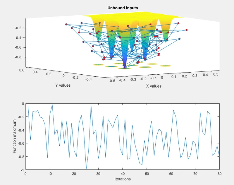
In the first study there are no lower and upper limits hence the GA does not the search space is between 0 and 1. Hence each time the program is executed different optimum values are are obtained as shown in the plot 2.

• STUDY 2

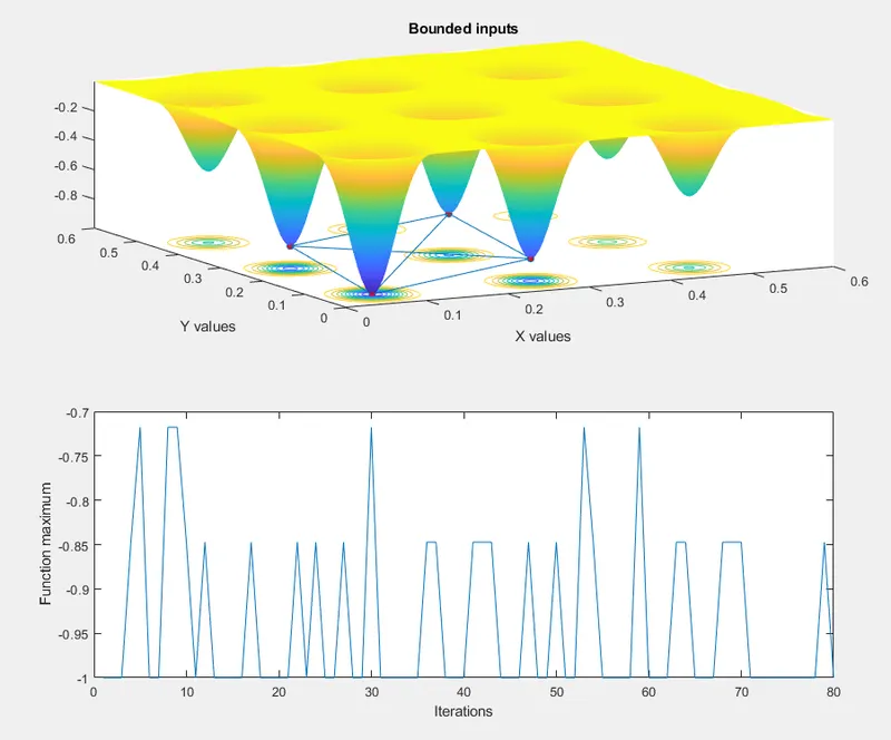
In the 2nd study lower and upper limits are included in the GA. Hence most of the maximum values obtained in each iteration varies between (-1) and (-0.7). This method narrows down the maximum values to 4 points as shown in the plot 1.

• STUDY 3

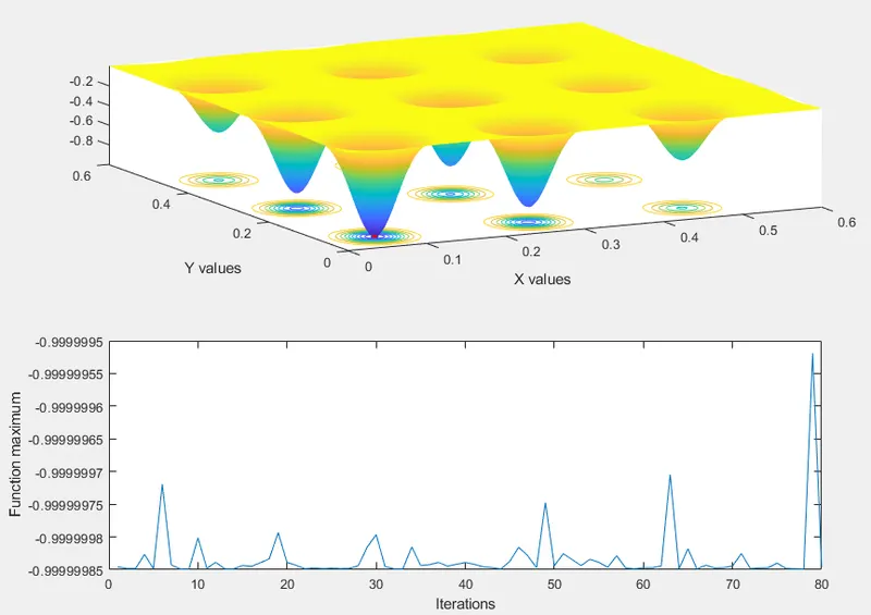
In the 3rd study the global maximum obtained is accurate and is narrowed down to a value of -0.999999 as shown in the graphs.

CONCLUSION :

• Optimised stagalmite function and global maxima of function is found successfully by using MATLAB.