Project
Aim:
To do a detailed study of Continuous Variable Transmission (CVT) using BAJA ATV vehicle and present our observations on it.
THEORY:
All-Terrain Vehicle:
An all-terrain vehicle (ATV), also known as a quad (cycle), three-wheeler, four-wheeler, or quadricycle, as defined by the American National Standards Institute (ANSI) is a vehicle that travels on low-pressure tires, with a seat that is straddled by the operator, along with handlebars for steering control. It is designed to handle a wider variety of terrain than most other vehicles.
BAJA ATV (SAE):
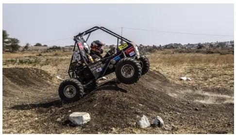
The BAJA SAE series is an event for undergraduate engineering students, organized globally by the Society of Automotive Engineers, USA. The event originated under the name of Mini-BAJA, In the year 1976 at the University of Carolina. Since then, the event has spanned six countries-USA, Mexico, South Africa, Korea, Brazil and India. The BAJA SAE tasks the students to design, fabricate and validate a single-seater four-wheeled off-road vehicle to take part in a series of events spread over a course of 3 days that test the vehicle for the sound engineering practices that have gone into it, the agility of the vehicle in terms of grade ability, speed, acceleration and manoeuvrability characteristics and finally its ability to endure that back-breaking durability test.
Continuous Variable Transmission (CVT):
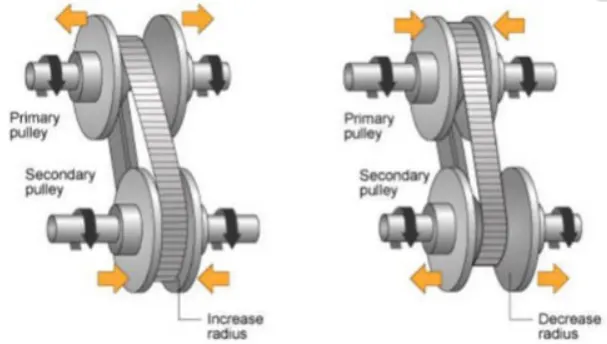
A Continuously Variable Transmission (CVT) is an automatic transmission that can change seamlessly through a continuous range of gear ratios. This contrasts with other transmissions that provide a limited number of gear ratios in fixed steps. The flexibility of a CVT with suitable control may allow the engine to operate at a constant RPM while the vehicle moves at varying speeds.
CVTs are used in automobiles, tractors, motor scooters, snowmobiles, and earthmoving equipment. The most common type of CVT uses two pulleys connected by a belt or chain, however, several other designs have also been used at times.
Blocks used:
1) Signal Builder:
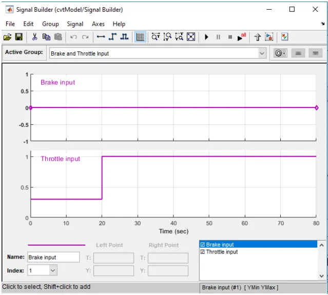
Signal Builder is used for giving input values of brake input and throttle input and it is connected with Generic Engine Block.
Where,
-Brake Input =0,
-Throttle Input= 0.3 for the first 20 sec, after 20-sec throttle input will be 1.
2) Generic Engine:
Represents a system-level model of spark-ignition and diesel engines suitable for use at the initial stages of modelling when only the basic parameters are available. Optional idle speed and red line controllers are included.
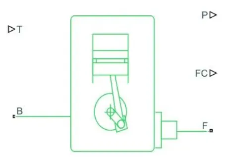
Connections F and B are mechanical rotational conserving ports associated with the engine crankshaft and engine block, respectively, connections P and FC are physical signal output ports through which engine power and fuel consumption rate are reported.
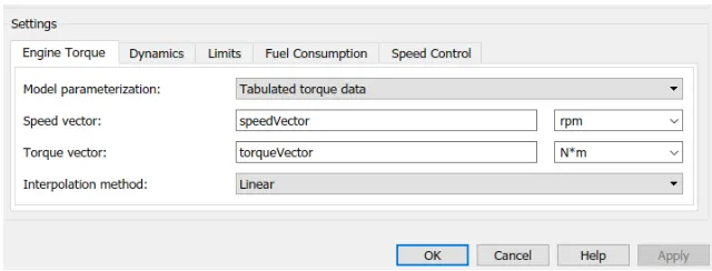
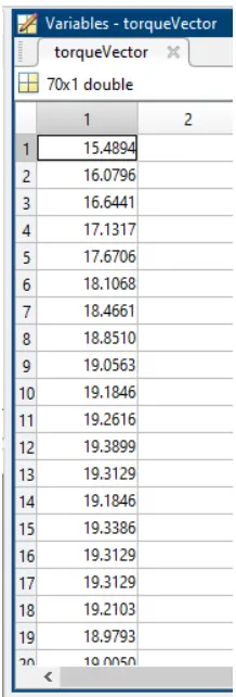
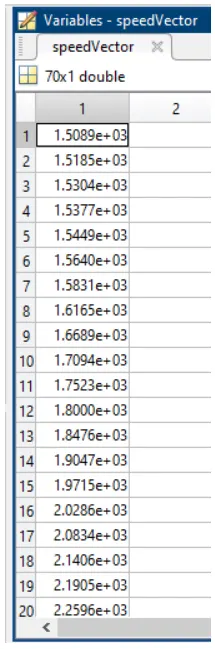
Torque vector and speed vector value is already assigned in the MATLAB program in an array data set.
3) Engine Sensor:
Engine Sensor is connected with Generic Engine. Engine Sensor contains Ideal Mechanical Rotational Sensor that converts as across variable measured between two mechanical rotational nodes into a control signal proportional to angular velocity or angle.
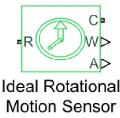
Connections R and C are mechanical rotational conserving ports and connections W and A are physical signal output ports for velocity and angular displacement, respectively.
4) Simple Gear:
The engine is connected to CVT with a simple gear ratio for Speed Reduction.
Continuously Variable transmission:
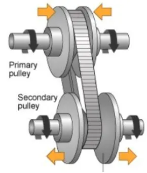
The main components of Continuously Variable Transmission (CVT) are given below:
- Primary Pulley
- Secondary Pulley
- Variator
- Belt
Note 1: If the Variator of the Primary Pulley goes outward and the Secondary pulley goes inward it will lead to Speed Reduction.
Rp < Rs
Note 2: If Variator of Primary Pulley goes inward and Secondary Pulley goes Outward it will lead to Overdrive.
Rp > Rs
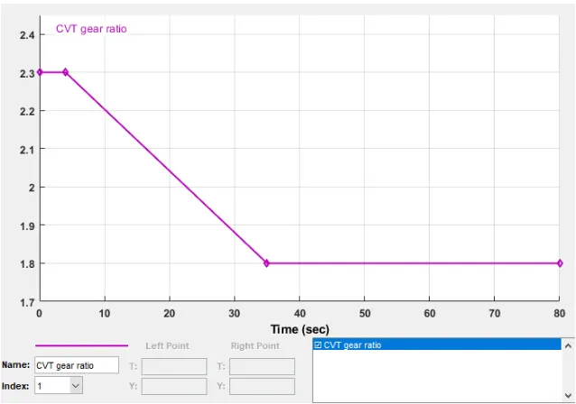
4a) CVT Ratio: (Signal Builder)
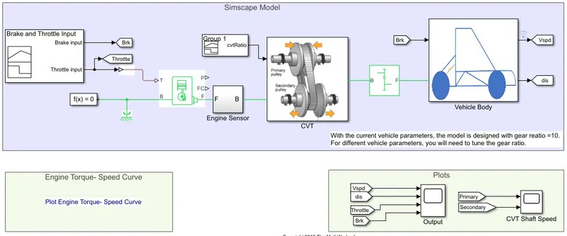
CVT Ratio Block is connected with CVT by giving random ratio values to get the value of velocity for those random CVT ratios.
5) Vehicle Body:
Represents a two-axle vehicle body in longitudinal motion. The block accounts for body mass, aerodynamics drag, road incline and weight distribution between axles due to acceleration and road profile. The vehicle can have the same or a different number of wheels on each axle. Optionally include pitch and suspension dynamics or additional variable mass and inertia. The vehicle does not move vertically relative to the ground.
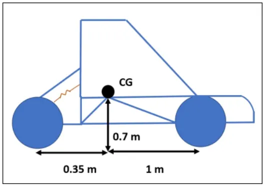
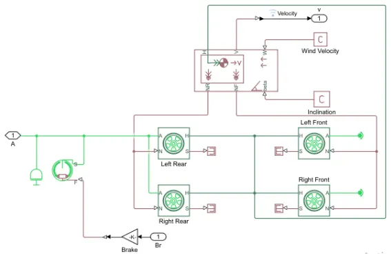
The vehicle Body contains Two Front Wheels and Two Rear Wheels which are connected with Inertia Output Shaft and a Double Shoe brake.
6) Double Shoe Brake:
The Double-shoe Brake block represents a frictional brake with two pivoted rigid shoes that press against a rotating drum to produce a braking action. The rigid shoes sit inside or outside the rotating drum in a diametrically opposed configuration. A positive actuating force causes the rigid shoes to press against the rotating drum. Viscous and contact friction between the drum and the rigid shoe surfaces cause the rotating drum to decelerate.
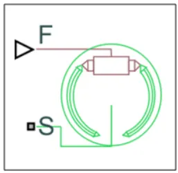
Port S is for the Rotational conserving port associated with the rotating drum shaft and F is for the Physical signal input port associated with the applied actuating force.
Other blocks:
- Simulink to PS Converter-To convert the Simulink signal to a Simscape environment
- Solver Configuration-To specify the solver parameters before starting the simulation
- Mechanical Reference-To make sure all the components are clamped to the ground
- PS to Simulink Converter- To convert Simscape Signal to Simulink environment
- Scope- To view the graph of the parameters for a better understanding
- Display-To view the calculated engine power
- Inertia-To represent the solid inertia
- Rotational Motion Sensor-To sense the rotational motion from the engine and give output as rpm
- Variable Gear Ration- To vary the speed according to the gear
- PS Terminator- Terminator for unconnected physical signal output
- PS Constant-generate constant physical signal
- Rotational Free End- for mechanical component (Tire)
- Vehicle Body-To represent the BAJA ATV model body
- Custom Measure Gauge- To measure the brake and throttle input
- Knob- To increase, decrease and vice-versa of throttle and brake inputs
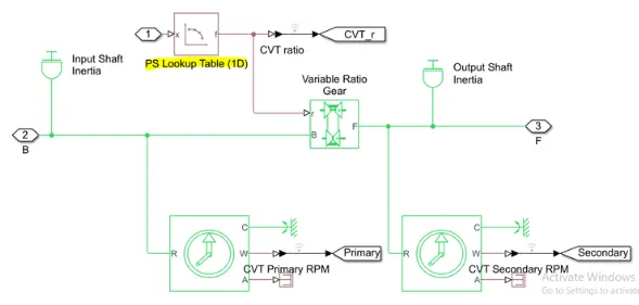
- Lookup Table- To insert the CVT values from the workspace
- Step- To increase or decrease an input value for a defining time interval
CASE STUDIES:
Study 1:
Case 1:
- BAJA ATV With CVT:
Result:
Engine Torque vs Speed Curve:
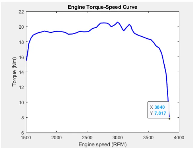
In the above plot maximum velocity reaches 3840 RPM. Vehicle speed depends on CVT Ration.
Vehicle Speed Plot:
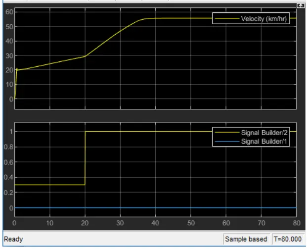
In the above plot, Brake Input is 0 and Throttle input is 0.3 for 20-sec Velocity will reach 20 and by increasing the Throttle input value to 1, the velocity value will increase and it reaches the maximum velocity
CVT Shaft Speed Plot:
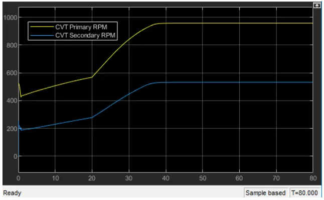
In continuously variable Transmission (CVT) Variator of the Primary pully goes inward and the Secondary pulley goes Outward which will lead to Overdrive. The Primary Pulley radius increases and the secondary pulley radius decreases. So, the speed of the Primary pulley is greater than the Secondary pulley.
Rp > Rs
Engine Speed:
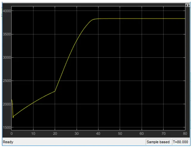
In the above plot, Brake Input is 0 and Throttle Input is 0.3 for 20 sec, Engine Speed will decrease at the beginning because of increasing gear ratio which increases the torque and by increasing the Throttle input value to 1, then Engine Speed value will increase and it reaches the maximum speed.
CASE-2:
2) ATV with CVT Using DASHBOARD:
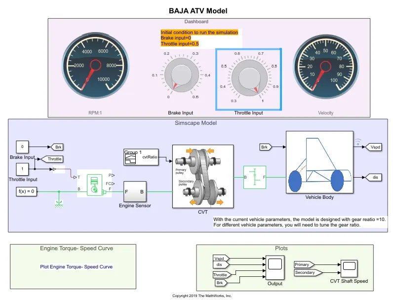
In the Above Simulink Model, RPM (speed) gauge, Brake input gauge, Throttle input gauge ND Velocity gauge is connected to the dashboard. Brake input is 0, Throttle input is 0.3 for an initial condition to run Simulation.
The dashboard is connected with BAJA All-terrain Vehicle using CVT in Simulink Model. With the help of Dashboard, variation in speed and Velocity will display in the rpm:1 gauge and Velocity gauge, while running the simulation.
RPM gauge refers to the speed of the primary & Secondary pulley and the Velocity gauge refers to the speed of the vehicle.
RESULT:
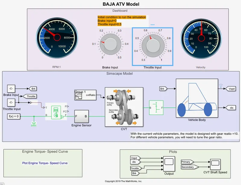
In the initial condition, the RPM:1 gauge shows 0 RPM and the velocity gauge shows 0 km/hr.
Giving time value as “inf” and Running the Simulation. While simulation is running, throttle input value & Brake Input Value can change in the Throttle input gauge & Brake Input gauge in the dashboard and will analyse the variation of RPM and velocity in the RPM gauge and velocity Gauge.
Vehicle Speed Plot:
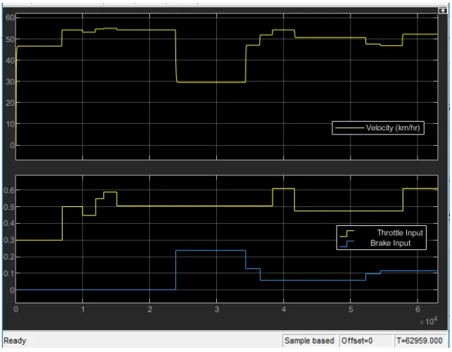
From the above Vehicle Speed Plot, observed that increasing the throttle input value, will increase the Velocity and increasing the brake input value will decrease the Velocity.
CVT shaft Speed Plot:
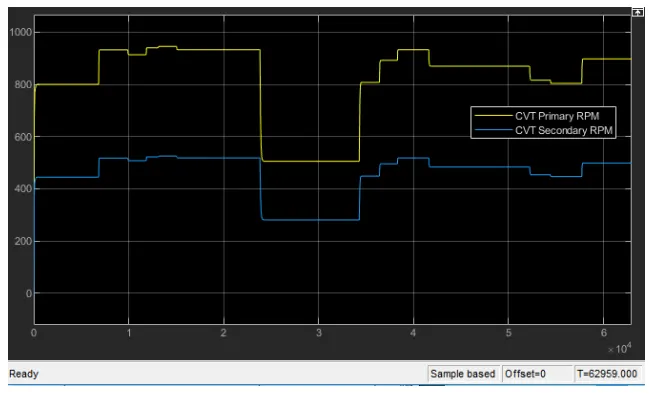
From the above CVT Shaft plot, observed that increasing the throttle input value, will increase the RPM of the Primary & Secondary Pulley and increasing the brake input value will decrease the RPM of the Primary & secondary Pulley.
ENGINE SPEED:
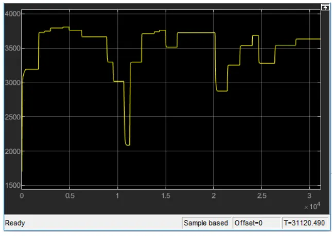
From the above engine Speed Plot, observed that increasing the throttle input value, will increase the Engine Speed and increasing the brake input value will decrease the Engine Speed.
STUDY-2:
CASE- 1:
- ATV with CVT: (Using lookup Table).
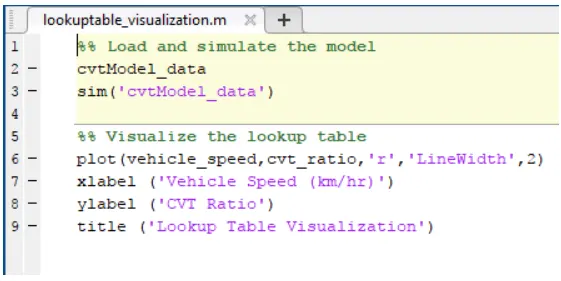
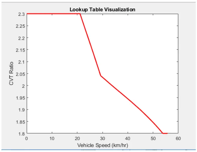
In the above model, Lookup table data has been assigned as input to the CVT instead of giving the CVT ratio. For Giving input of LOOK up table by creating a program in the MATLAB and Data has been assigned as input to the CVT.
Look Up Table Program in MATLAB:
Code for Lookup Table
WORKSPACE:
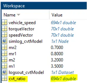
Look Up Table data has been assigned as the CVT ratio in the workspace.
GIVING INPUT TO CVT USING LOOKUP TABLE:
After creating Look Up Table data, give data, and give the data as input to the CVT.
Result:
Look Up Table Visualization Plot:
CVT Ratio Plot: (Look Up Table Data).
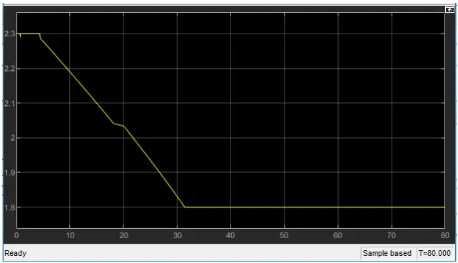
The above plot shows the value of the Look-Up Table input data given to the CVT.
Vehicle Speed Plot:
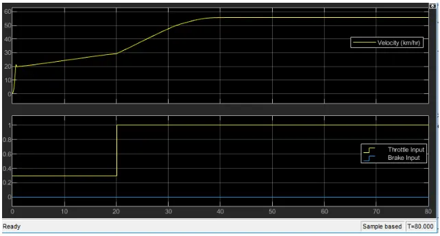
In the above Plot, the Brake input is 0 and Throttle Input is 0.3 for 20-sec Velocity will reach 20 and by increasing the Throttle input value to 1, the Velocity will increase and it reaches the maximum velocity.
CVT Shaft Speed Plot:
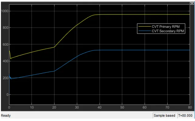
In Continuously Variable Transmission (CVT) Variator of the Primary pulley goes inward and Secondary Pulley goes Outward which will lead to Overdrive. Primary Pulley radius increases and Secondary Pulley radius decreases. So, the Speed of the Primary pulley is greater than the Secondary Pulley.
Rp > Rs
Engine Speed:
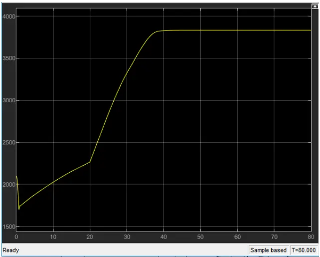
In the above plot, the Brake input is 0 and the Throttle input 0.3 for 20 sec, Engine Speed ill decrease at the beginning because of the increasing gear ratio which increases the torque and by increasing the Throttle input value to 1, the Engine speed value will increase and it reaches the maximum speed.
CASE-2:
- ATV with CVT with DASHBOARD: (Using Look-Up Table)
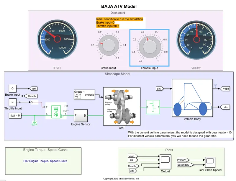
In the above Simulink Model, RPM (speed) gauge, Brake Input gauge, Throttle Input and velocity gauge are connected in the dashboard Brake input is 0, Throttle input is 0.3 for the initial condition to run the simulation.
In the above model, lookup table data has been assigned as input to the CVT instead of giving the CVT ratio. For Giving input of lookup table by creating a program in the MATLAB and Data has been assigned as input to the CVT.
Result:
CVT Ratio Plot: (Lookup Table Data).
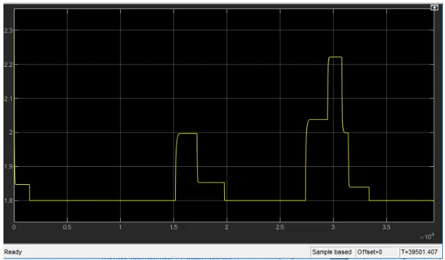
In the above plot, the CVT Ratio will vary by changing the Throttle gauge. If throttle value increases CVT ratio decreases. If the Throttle value decreases CVT Ratio increases.
Vehicle Speed Plot:
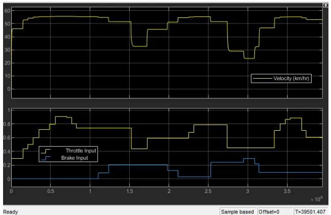
From the above Vehicle Speed Plot, observed that increasing the throttle input value, will increase the Velocity and increasing the brake input will decrease the velocity.
CVT Shaft Speed Plot:
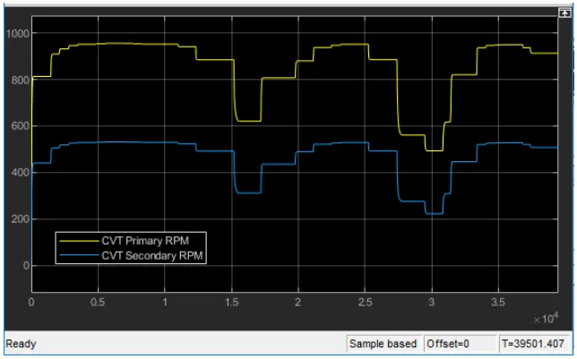
From the above CCVT Shaft Speed plot, observe that by increasing the throttle input value. It will increase the RPM of the Primary and Secondary Pulley and by increasing the brake input value it will decrease the RPM of the Primary and Secondary Pulley.
Engine Speed Plot:
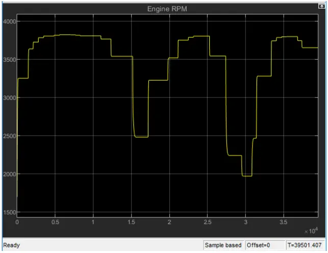
From the above Engine Speed plot, observed that increasing the throttle input value, will increase the Engine Speed and increasing the brake input value will decrease the Engine Speed.
Conclusion:
System-level Simulation of a BAJA All-terrain vehicle without using Look Up Table is done and the results are plotted.
System-level Simulation of a BAJA All-terrain vehicle using Look Up Table is done and the results are plotted.
All the results are satisfactory.