Project
AIM:
To carryout system level simulation of Baja All Terrain Vehicle (ATV) and analyse the results.
Objective:
Analyse each individual block used to built the system model.
Understanding realationship among the blocks & thereby how the process flowing from one block to other.
Analyse the results & know how a system can be modeled in different ways using Simulink, Simscape, and Simscape Driveline.
Theory:
What is an ATV ?
An all-terrain vehicle (ATV) is defined as a motorized off-highway vehicle designed to travel on four low-pressure or non-pneumatic tires, having a seat designed to be straddled by the operator and handlebars for steering control. ATVs are subdivided into two types as designated by the manufacturer. Type I ATVs are intended by the manufacturer for use by a single operator and no passenger. Type II ATVs are intended by the manufacturer for use by an operator and a passenger, and are equipped with a designated seating position behind the operator. Similarly, riders must also consider the various ATV sizes.
An all-terrain vehicle (ATV), as the name implies, it is designed to handle a wider variety of terrain than most other vehicles. Although it is a street-legal vehicle in some countries, it is not street-legal within most states, territories and provinces of some countries
The ATVs are not road legal in India and they cannot be registered through the RTO. Which means they cannot be used on public roads. Such off-road vehicles can only be used in private properties like farms or racing tracks but not on public roads
Baja SAE
Baja SAE is a Collegiate Design Series competition run by the Society of Automotive Engineers International (SAE International).Teams of students from universities all over the world design and build small off-road cars. The cars all have engines of the same specifications.
The goal in Baja SAE racing is to design, build and race off-road vehicles that can withstand the harshest elements of rough terrain. The vehicles used in Baja SAE racing are often similar in appearance to dune buggies.
Baja ATV model:
For model files - Click Here
This contains a set of models created with Simulink, Simscape, and Simscape Driveline.
More specifically, the file contained includes BAJA ATV model with Continuously Variable Transmission(CVT).
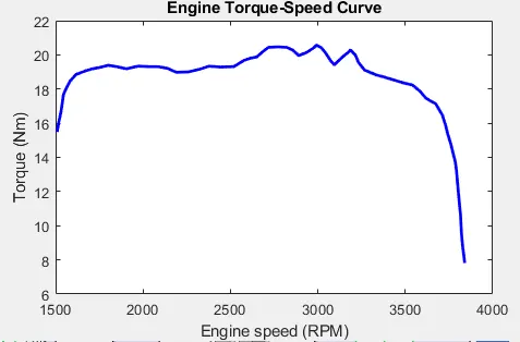
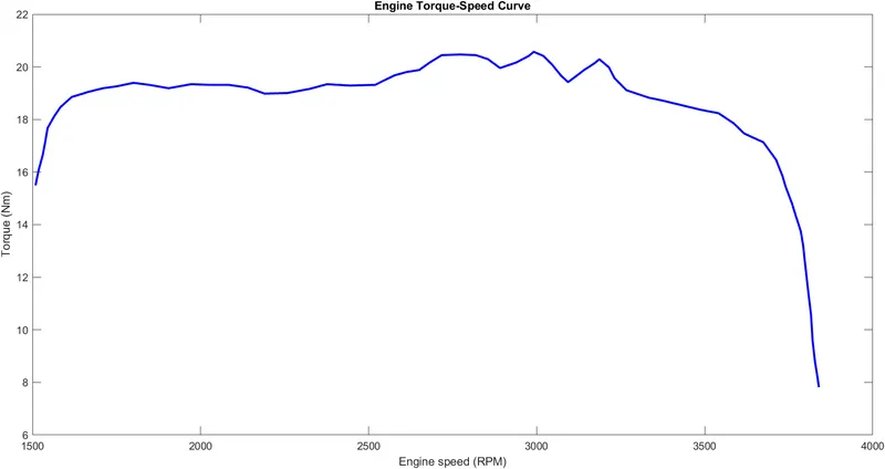
The engine data used in the model is provided as an image which shows the Engine Speed (RPM) Vs Torque curve.
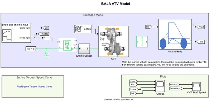
We can look into the model as 3 major blocks/subsystems
1) Engine
2) CVT-Continuous Variable Transmission &
3) Vehicle body
1) Engine :
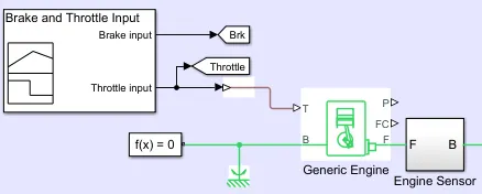
Generic Engine block:
The Generic Engine block represents a general internal combustion engine. This block is a suitable generic engine for spark-ignition and diesel. Speed-power and speed-torque parameterizations are provided. A throttle physical signal input specifies the normalized engine torque. Optional dynamic parameters include crankshaft inertia and response time lag. A physical signal port outputs the engine fuel consumption rate based on the fuel consumption model that you choose. Optional speed and redline controllers prevent engine stall and enable cruise control.
Ports :
T - Physical signal port representing Engine torque demand as a fraction of maximum possible torque
B - Mechanical rotational conserving port associated with the engine block. This is the base port. The engine block is the physical body that contains the piston cylinders
F - Mechanical rotational conserving port associated with the engine crankshaft. This is the follower port of engine. The crankshaft transmits the power generated from the combustion process. Typically, you attach a clutch and transmission at this port
FC - Physical signal port represnting Fuel consumed by the engine, in kg/s
P - Power produced by the engine, in W
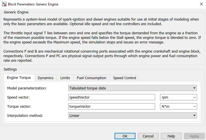
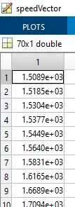
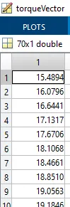
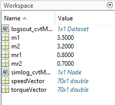
'SpeedVector' and 'TorqueVectors' shown above as reference from Matlab workspace are collected from the bellow image "Engine Torque-Speed Curve" using Matlab GRABIT function and assigned from workspace
Solver block:
Simulink® provides a set of programs called solvers. Each solver embodies a particular approach to solving a model. A solver applies a numerical method to solve the set of ordinary differential equations that represent the model. Through this computation, it determines the time of the next simulation step.
Reference block:
The Mechanical Rotational Reference block represents a reference point, or frame, for all mechanical rotational ports. All rotational ports that are rigidly clamped to the frame (ground) must be connected to a Mechanical Rotational Reference block.
Here a Solver Cinfiguration block "f(x)=0" & "Mechanical Rotational reference" are connected to the base port B of the engine block
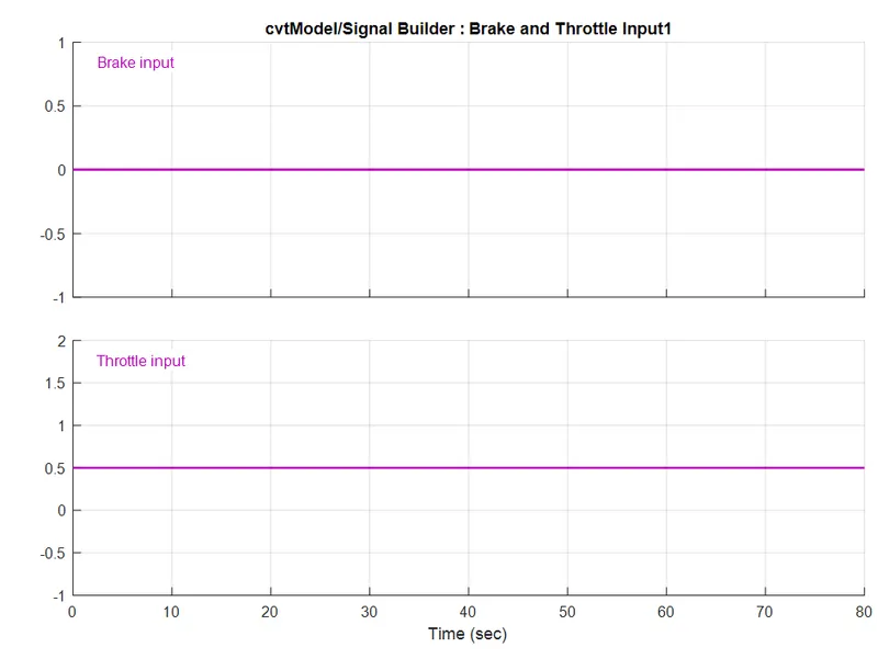
Signal Builder block:
A Subsystem block named "Engine Sensor" is used to measure RPM using a Ideal Rotational Motion Sensor block and a PS-Simulink converter block to convert measured angular velocity physical signal to simulink signal that serves as input to Scope(Engine RPM)
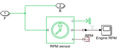
Ideal Rotational Motion Sensor:
The Ideal Rotational Motion Sensor block represents an ideal mechanical rotational motion sensor, that is, a device that converts an across variable measured between two mechanical rotational nodes into a control signal proportional to angular velocity or angle. You can specify the initial angular position (offset) as a block parameter.
The sensor is ideal since it does not account for inertia, friction, delays, energy consumption, and so on.
Connections R and C are mechanical rotational conserving ports that connect the block to the nodes whose motion is being monitored. Connections W and A are physical signal output ports for velocity and angular displacement, respectively.
2) CVT:
Continuously variable transmission (CVT):
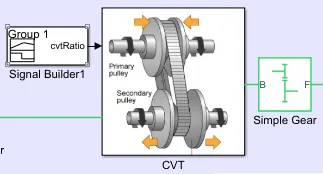
Continuously variable transmission (CVT) is an automatic transmission that can change seamlessly through a continuous range of gear ratio. This contrasts with other transmissions that provide a limited number of gear ratios in fixed steps. The flexibility of a CVT with suitable control may allow the engine to operate at a constant RPM while the vehicle moves at varying speeds.
CVTs are used in automobiles, trctors,motor scooters, snowmobiles,bicycle and earthmoving equipments.
The most common type of CVT uses two pulleys connected by a belt or chain; however, several other designs have also been used at times.
In the above figures,we can see the CVT mechanism consisting of a primary pulley, secondary pulley and a belt connecting the both.
Low gear : When primary pulley/drive pulley is widening and secondary pulley is narrowing
High gear: When primary pulley/drive pulley is narrowing and secondary pulley is widening
Belt : Here the belt transfering the torque from one pulley to the other over the continuous variable transmission.
In our model, a variable ratio transmission block is used to represent the CVT
Intertia of the primary & secondary pulleys are represented using Inertia block (This block represents an ideal mechanical rotational inertia)
Velocity of primary and secondary shafts are measured using Ideal Rotational Motion Sensor block and a PS-Simulink converter block to convert measured angular velocity physical signal to simulink signal that serves as input to Scope(CVT Primary RPM & CVT secondary RPM)
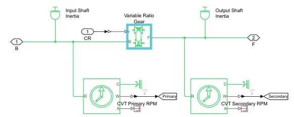
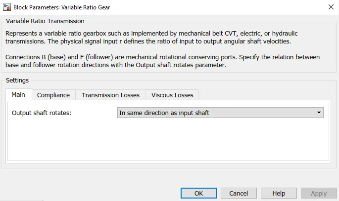
CVT/Variable Ratio Gear block with ports B, r & F representing
B - Mechanical rotational conserving port associated with the base driveshaft, it is directly connected to engine shaft
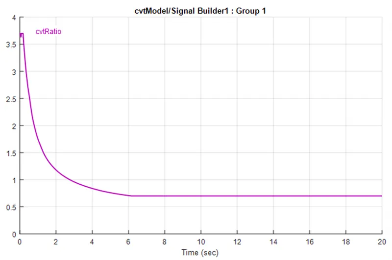
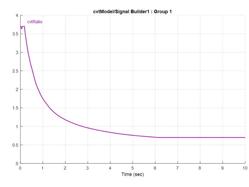
r - Physical signal port associated with the input to output shaft ratio. Here another signal builder block is used to provide CVT Ratio to the Variable Ratio transmission block, as shown in above fig.
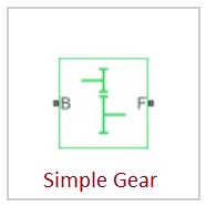
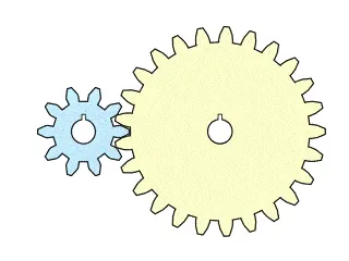
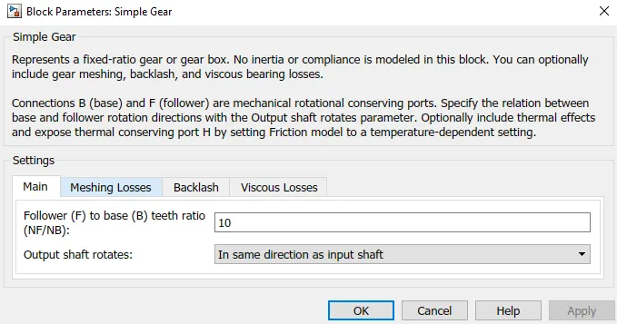
F - Mechanical rotational conserving port associated with the follower driveshaft. It is connected to a simple gear block with gear ratio of 10
3) Vehicle body:
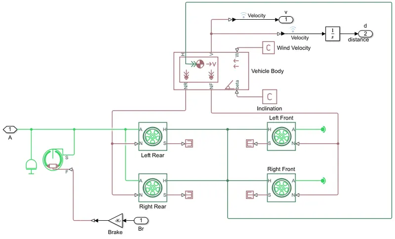
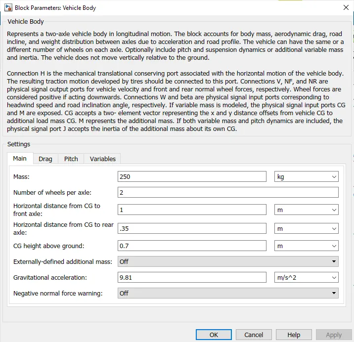
Vehicle Body block
represents two-axle vehicle with longitudinal dynamics and motion and adjustable mass, geometry, and drag properties
The vehicle can have the same or a different number of wheels on each axle. For example, two wheels on the front axle and one wheel on the rear axle. The vehicle wheels are assumed identical in size. The vehicle can also have a center of gravity (CG) that is at or below the plane of travel.
The block accounts for body mass, aerodynamic drag, road incline, and weight distribution between axles due to acceleration and road profile. Optionally include pitch and suspension dynamics. The vehicle does not move vertically relative to the ground.
The block has an option to include an externally-defined mass and an externally-defined inertia. The mass, inertia, and center of gravity of the vehicle body can vary over the course of simulation in response to system changes.
W- headwind speed, m/s
beta - road incline angle, rad
V- vehicle longitudinal velocity
NF- normal force on the front axle. Wheel forces are considered positive if acting downwards
NR- normal force on the rear axle. Wheel forces are considered positive if acting downwards.
H- Conserving port associated with the horizontal motion of the vehicle body. Connect tire traction motion to this port.
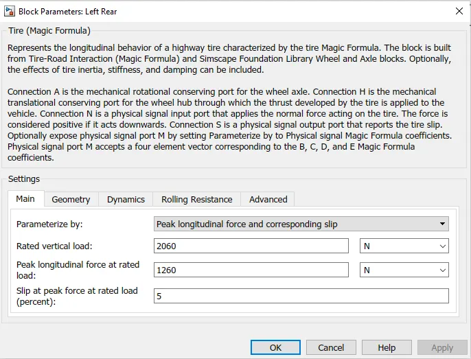
Tire block:
The Tire (Magic Formula) block models a tire with longitudinal behavior given by the Magic Formula [1], an empirical equation based on four fitting coefficients. The block can model tire dynamics under constant or variable pavement conditions.
To increase the fidelity of the tire model, you can specify properties such as tire compliance, inertia, and rolling resistance. However, these properties increase the complexity of the tire model and can slow down simulation. Consider ignoring tire compliance and inertia if simulating the model in real time or if preparing the model for hardware-in-the-loop (HIL) simulation.
The Tire (Magic Formula) block models the tire as a rigid wheel-tire combination in contact with the road and subject to slip. When torque is applied to the wheel axle, the tire pushes on the ground (while subject to contact friction) and transfers the resulting reaction as a force back on the wheel. This action pushes the wheel forward or backward. If you include the optional tire compliance, the tire also flexibly deforms under load.
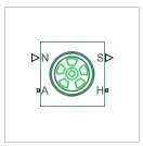
N-normal force acting on the tire
S-relative slip between the tire and road
A- the axle that the tire sits on
H-wheel hub that transmits the thrust generated by the tire to the remainder of the vehicle
Double Shoe Brake block:
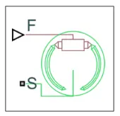
The Double-Shoe Brake block represents a frictional brake with two pivoted rigid shoes that press against a rotating drum to produce a braking action. The rigid shoes sit inside or outside the rotating drum in a diametrically opposed configuration. A positive actuating force causes the rigid shoes to press against the rotating drum. Viscous and contact friction between the drum and the rigid shoe surfaces cause the rotating drum to decelerate.
Double-shoe brakes provide high braking torque with small actuator deflections in applications that include motor vehicles and some heavy machinery. The model employs a simple parameterization with readily accessible brake geometry and friction parameters.
F- applied actuating force
S- rotating drum shaft
n-D Lookup table:
The 1-D, 2-D, and n-D Lookup Table blocks evaluate a sampled representation of a function in N variables
y=F(x1,x2,x3,...,xN)
where the function F can be empirical. The block maps inputs to an output value by looking up or interpolating a table of values you define with block parameters. The block supports flat (constant), linear (linear point-slope), Lagrange (linear Lagrange), nearest, cubic-spline, and Akima spline interpolation methods. You can apply these methods to a table of any dimension from 1 through 30.
PS- Lookup table:
he PS Lookup Table (1D) block computes an approximation to some function f=f(x) given data vectors x and f. Both the input and the output are physical signals.
The length of the x and f data vectors provided to this block must match. Also, the x data vector must be strictly monotonic, either increasing or decreasing.
You define the lookup table by specifying the Table grid vector parameter as a 1-by-n vector (x data vector) and the Table values parameter as a 1-by-n vector (f data vector). The block generates output based on the input values using the selected interpolation and extrapolation methods. You have a choice of two interpolation methods and two extrapolation methods. You also have an option for the block to issue an error if the input signal value is outside the table grid vector range.
Plotting Table Data
Plotting a lookup table lets you visualize the data before simulating the model, to make sure that the table is correct. The plot reflects tabulated data specified for the block, as well as the selected interpolation and extrapolation options.
Other Blocks include:
Intertia block - Rotational inertia of the vehicle body
Gain- To rise the effect of input brake
PS Constant - to provide inclined angle and windspeed inputs to the vehicle body blcok
PS-simulink & Simulink-PS converters: to converts the signals
Integrator - to calculate distance travelled from the vehicle velocity
Scope- to display the results
Inport,Outport, from & Goto- to connect signals from one sub system to other
PS Terminator - to specify the PS ports that are intentinally left unused.
Step signal- to provide break and throttles
Knob - to provide variable break and throttles in real time i.e while simulation is running
Circular gauge - to visualise engine RPM and vehivle speed while simulation is running
To workspace - to assign CVT ratio and vehicle speed vectors to workspace
Simulating the model files:
1a) cvtModel
Contains Simscape model of BAJA ATV with Continous Variable Transmission
CVT ratio provided to CVT block using signal builder
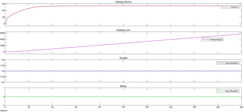
With a throttle of 0.5 and Brake=0, the vehicle taken about 40sec to reched its maximum speed, and the distance travelled by the vehicle in 200sec is 2834m
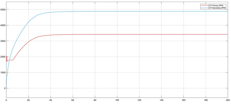
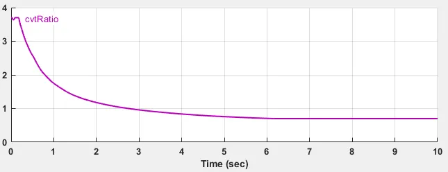
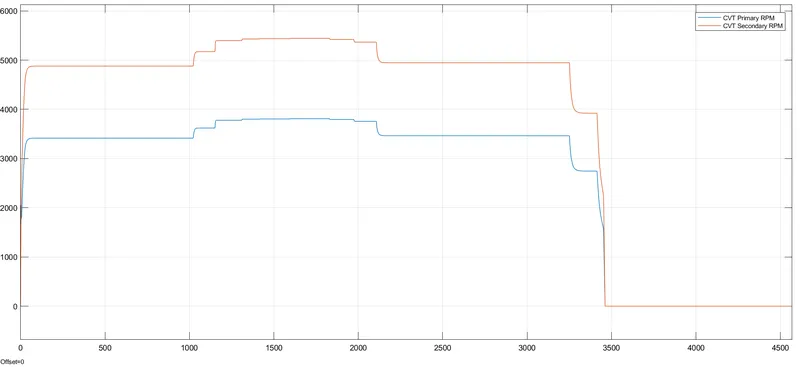
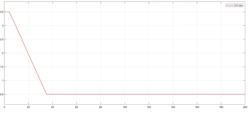
From the bellow plot and CVT ratio input graph, it is observed that fraction of Primary shaft RPM to secondary shaft RPM of CVT is matching with the CVT ratio signal provided at the input.
and also observed that CVT primary shaft RPM following the engine RPM and vehicle speed following CVT seocndary RPM.
With the use of CVT function, CVT secondary producing smooth transition as onserved from the bellow plot.
Engine RPM:
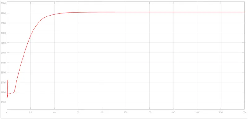
Plotted engine Torque-speed characteristic curve matching with the input speed & torque vectors provided as input from workspace. And this plot is same for all the models.
1b) cvtModel_dashboard
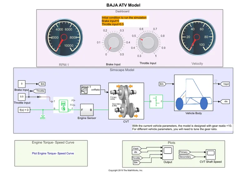
The model is similar to, "cvtModel" with addition of dashboards
In this model during simulation, we variedthrottle input to engine and brake input using knob and Engine RPM and Vehicle speed are observed using circular gauges.
Intial conditions brake=0,throttle=0.5
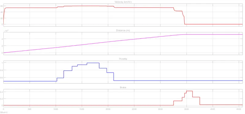
Bellow plot showing how the vehicle speed responding with varying input throttle and application of barke to wheels
Vehicle velocity along with input throttle and brake input:
CVt Ratio input :
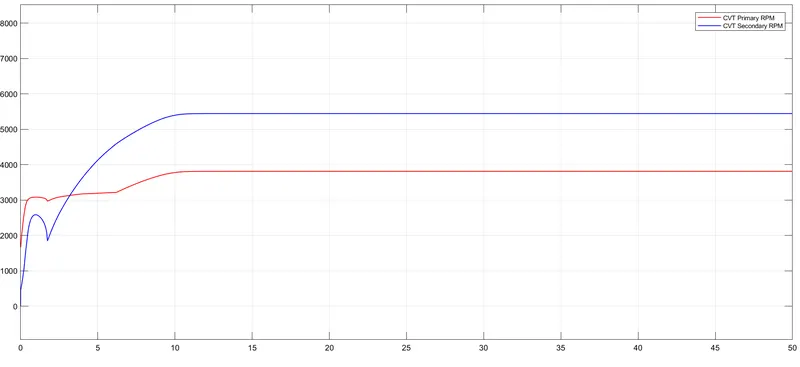
CVT Shaft speed:
Engine RPM:
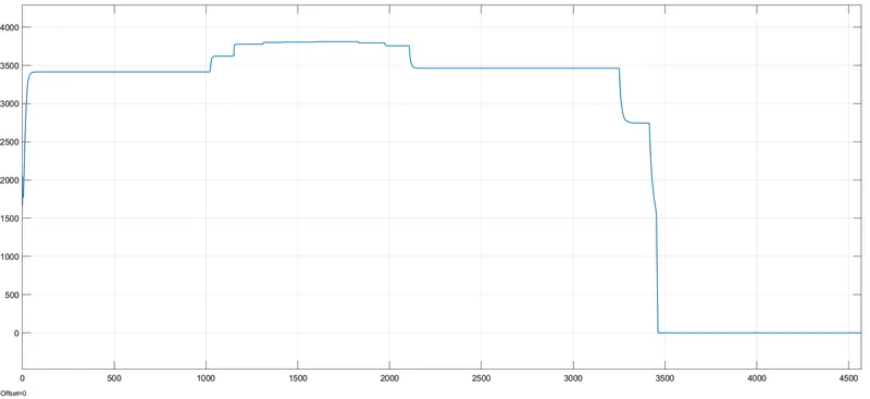
Here in this model we observe the variation in Engine RPM, CVT primary and secondary shafts RPM as a result of variation in Engine throttle and application of brake
2_Models_LookupTable
2a) cvtModel_cvtratio_rpm
Contains model based on cvt ratio and engine rpm lookup table
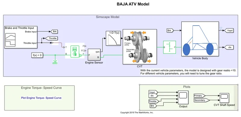
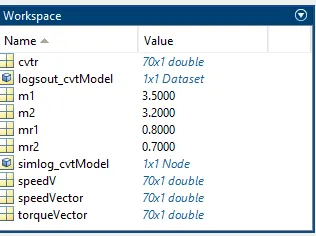
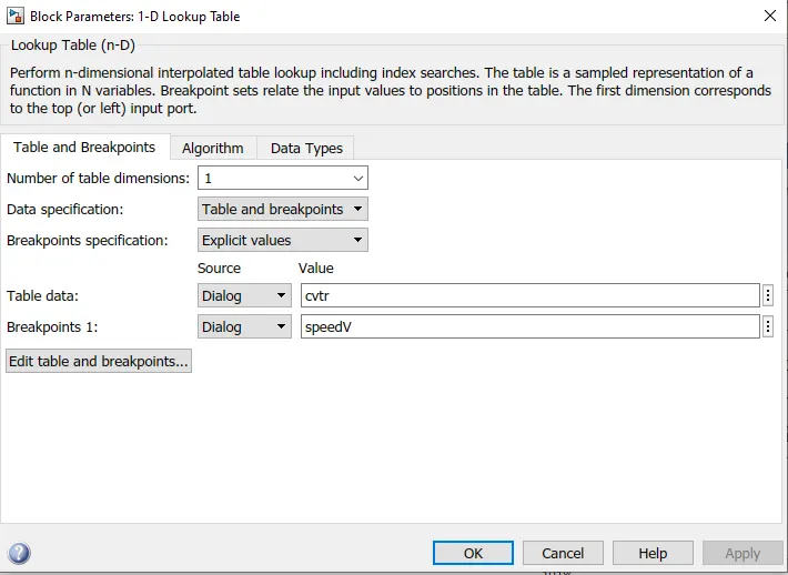
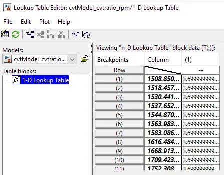
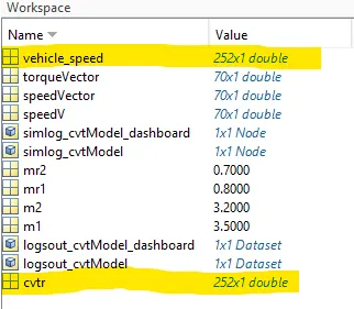
Vehicle speed and CVT ratio are logged into workspace and assigned in 1D look up table
Lookup table data:
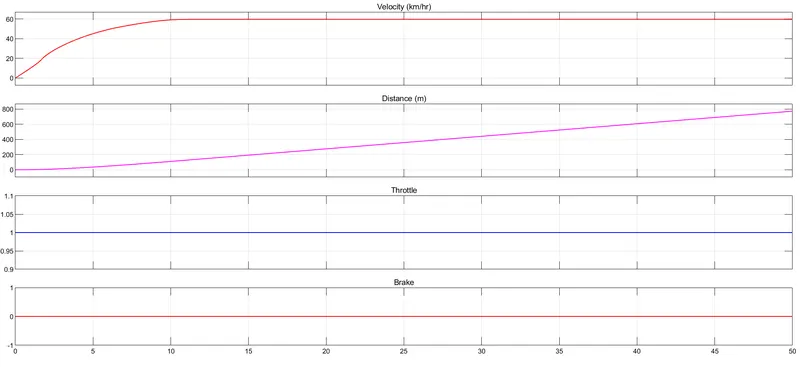
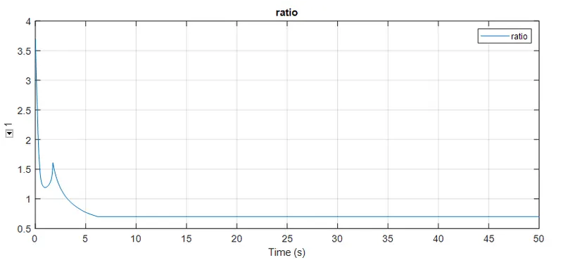
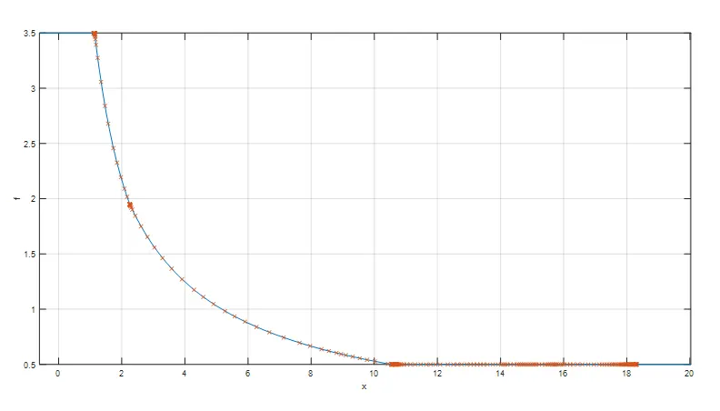
Here in the following plots, we can observe that vehicle speed as a function of CVT ratio
With an initial & continuos throttle of 1 ,and no brake applied, Vehicle reached its maximum speed in 10sec
While the CVT ratio is mantained constatnt , the vehicle maintined its maximum speed according to the applied CVT ratio
CVT ratio from 1D Lookup table :
Here is the CVT shaft RPM plot :
ii) cvtModel_mapped
Contains Simscape model of BAJA ATV with Continous Variable Transmission where the CVT ratio varies based on 1D lookup table.
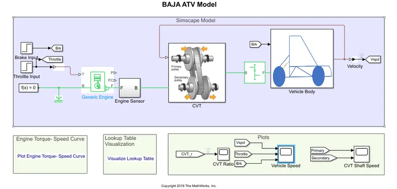
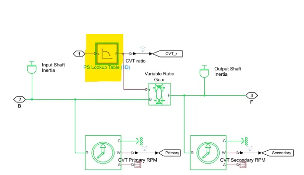
This model is same as the erlier but the difference is here we are using 'PS-lookup table' from Simscape instead of the 'n-D lookup table' from simulink in the previous one and here we provided vehicle velocity as input
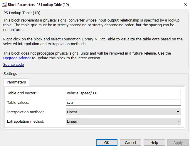
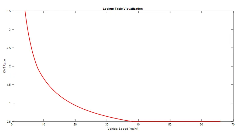
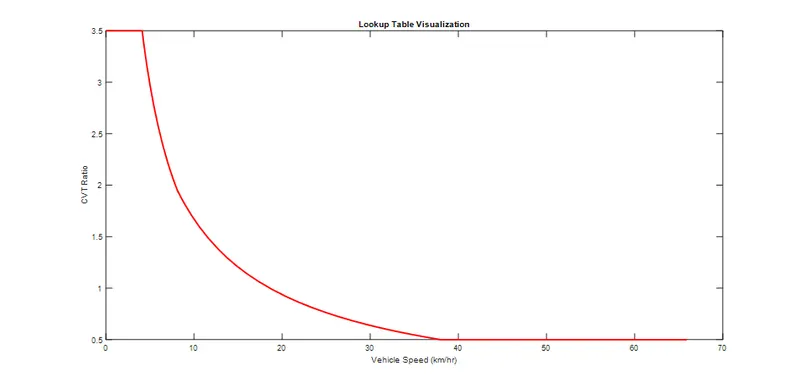
Here is the ploted lookup table from the data provided
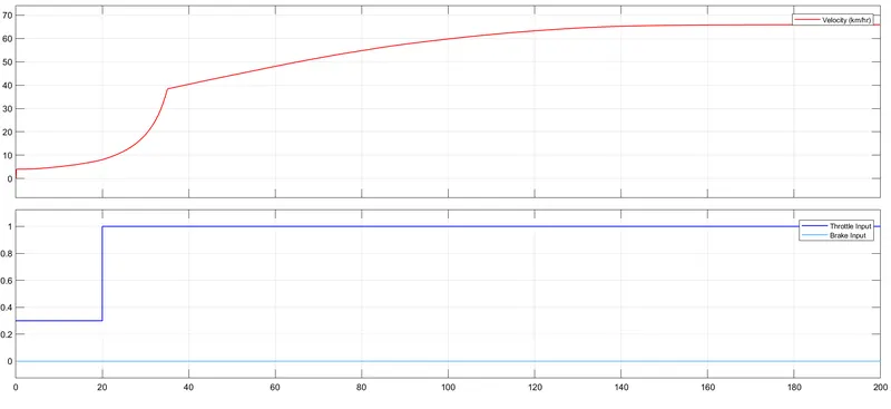
Here throttle maintained at 0.3 till first 20sec and then rised to 1 till the end of simulation and brake kept at 0
By observing the bellow plots vehicle speed is inline with the CVT's secondary shafts's RPM
CVT ratio:
CVT shaft Speed:
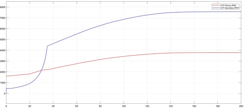
By observing the above two, ratio of primary shaft RPM to secondary shaft RPM is matching with the CVt ratio at that time instant.
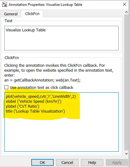
Here is the lookup table visualization program using Annotation:
cvtModel_dashboard_mapped
The model is similar to, "cvtModel_mapped" with addition of dashboards.
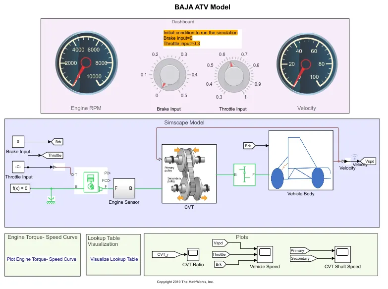
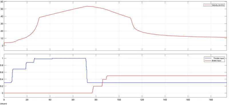
With initaial throttle of 0.3 and brake=0, started the simulation and while simulation is running throttle input to engine and brake applied are varied as shown in bellow plot.
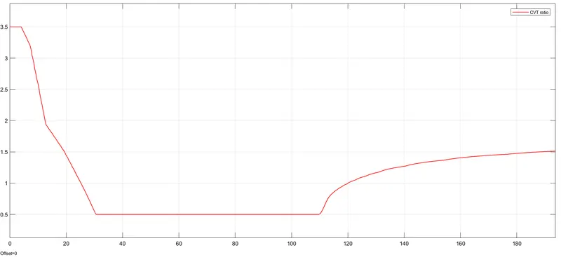
CVt ratio as a function of vehicle velocity:
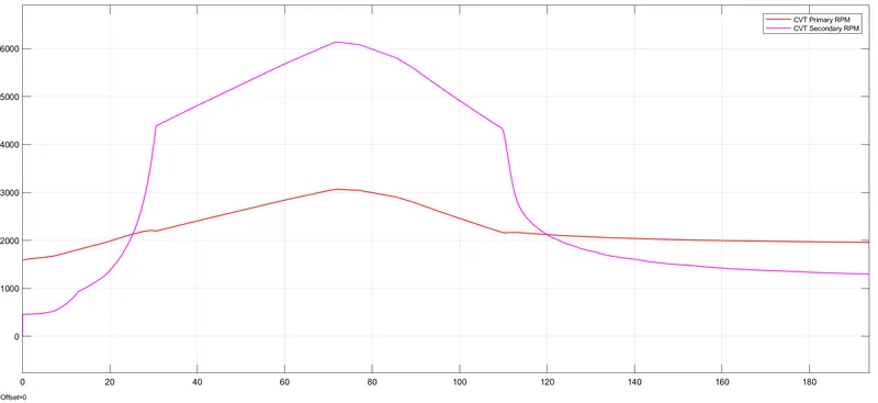
CVt shaft speed :
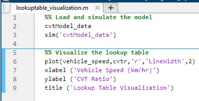
lookuptable_visualization
Script to load and run the model, "cvtModel_data". and to plot the lookup table
Conclusion:
Thus , we simulated different models of BAJA ATV and from the above results, we can infer that
-Vehicle speed, CVT Shaft RPM & Engine RPM are directly proportional to input throttle to engine & inversely proportional to brake applied.
-CVT ratio as a Signal builder function, as a function of engine RPM and as a function of vehicle speed using Lookup tables are simulated even in realtime and its results are analised.
- Finally we learn how can we built a (BAJA ATV) model in different ways using Simulink,simscape & simscape driveline environment and how to ineract with it in realtime and different affects are noticed.