Project

All Terrain Vehicle (ATV) Simulink Project

Aim :- To Study And Analyse The Different Cases Of BAJA All Terrain Vehicle (ATV) Model Using Simulink

OBJECTIVES :-

• To prepare technical report explaining models and their blocks
• To study different model properties
• To understand and comment on results

CASES STUDIED :-

1. BAJA ATV model – Without dashboard (cvtmodel)
2. BAJA ATV model – Data Extraction (cvtmodel_data)
3. BAJA ATV model – With Dashboard (cvtmodel_dashboard)
4. BAJA ATV model – Mapped Lookup Table Without Dashboard (cvtmodel_mapped)
5. BAJA AVT model – Mapped Lookup Table with Dashboard ( cvtmodel_dashboard_mapped)

INTRDUCTION : -

All Terrain Vehicle (ATV) :-

ATV also known as Light Utility Vehicle, a quad bike as defined by The American National Standards Institute(ANSI). ATV is an vehicle that travels on low pressure tries, with a seat that is straddled by the operator along with the handle bars for steering control.

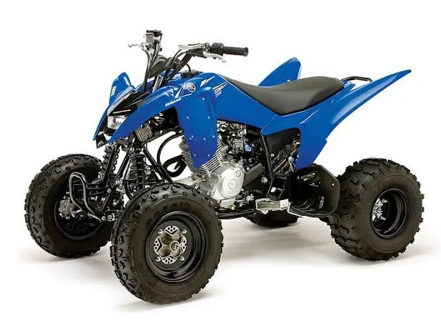
By current ANSI definition, ATV are intended for use by a single operator, although some companies have developed ATV s intended for use by operator and one passenger.

Continuously Variable Transmission (CVT) :-

CVT is an automatic transmission that can change seamlessly through a continuous range of gear ratio. This contrasts with other transmissions that provide a limited number of gear ratios in the fixed step. The flexibility of CVT with suitable control may allow the engine to operate at a CONSTANT RPM while the vehicle moves at varying speed.

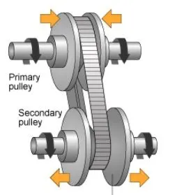
The most common type of CVT uses two pulleys connected by a belt or chain as shown above. However, several other designs are also used at times. CVT transmission is used to improve fuel efficiency and are more dependable than typical automatic gearboxes.

MAIN BLOCK USED :-

Vehicle Body Block -

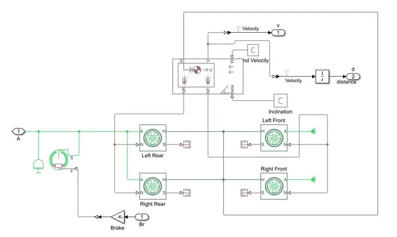
The vehicle body is a simscape block used as ATV vehicle body , that represents a two axle vehicle body in longitudinal motion. The vehicle have same or different numbers of wheels on each axle.

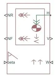
Where,

H = Input port for headwind speed (m/s)

Beta = Input port for road incline angle (rad)

V = output port for longitudinal velocity in the vehicle frame (m/s)

NF = output port for normal force on the front axle, wheel forced are consider positive if acting downwards (N)

NR = output port for normal force on the rear axle, wheel forced are consider positive if acting downwards (N)

The block accounts for body mass, aerodynamic drag, road incline weight distribution due to between axles due to acceleration and road profile.

Vehicle body subsystem –

Generic Engine :-

This block represents a general internal combustion engine for our ATV model . This is a suitable generic engine for spark ignition and diesel.

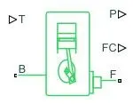
The generic block uses a programmed relationship between torque and speed that is modulated by the throttle signal.

where,

T = throttle input port for engine

B = Mechanical rotational conserving port associated with the engine block

F = Engine Crankshaft associated with rotational conserving port

P = instantaneous power output port for engine (W)

FC = This port is used to take a value of fuel consumed by the engine (kg)

RATIO TRANSMISSION GEAR (CVT) :-

The Variable Ratio Transmission block accepts the continuously varying gear ratio as a physical signal Simulink signal through the extra physical signal input labeled r.

Signal builder block input to CVT

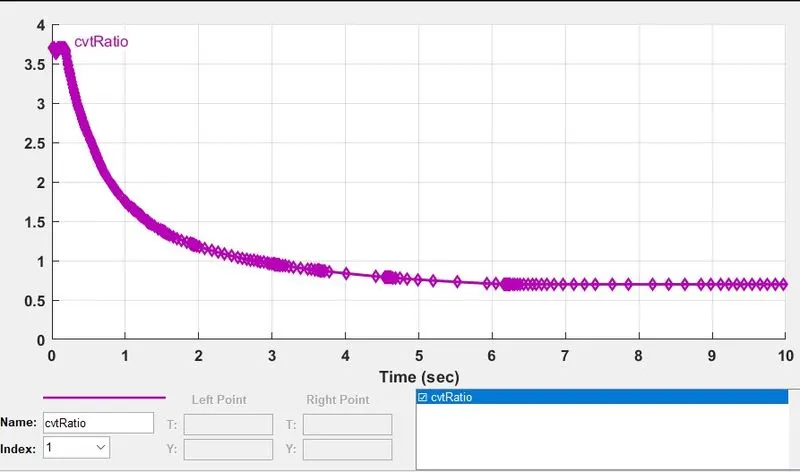
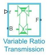
The gear ratio between the follower (F) and the base (B) is steadily increased or decreases .

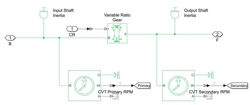
CVT subsystem

DOUBLE SHOE BRAKE :-

The Double-Shoe Brake block represents a frictional brake with two pivoted rigid shoes that press against a rotating drum to produce a braking action. The rigid shoes sit inside or outside the rotating drum in a diametrically opposed configuration. A positive actuating force causes the rigid shoes to press against the rotating drum. Viscous and contact friction between the drum and the rigid shoe surfaces cause the rotating drum to decelerate.

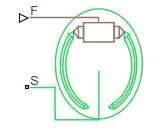
Double-shoe brakes provide high braking torque with small actuator deflections in applications that include motor vehicles and some heavy machinery. The model employs a simple parameterization with readily accessible brake geometry and friction parameters.

CASE 1 : BAJA ATV model – without dashboard (cvtmodel)

This is the main and basic model of BAJA ATV . where, signal builder block is used generate Brake and Throttle signal to drive and stop the ATV. Generic Engine is a simscape block Then with the help of Simulink to physical signal converter the throttle signal is given to T port of generic engine block. After that the output of engine is connected to engine sensor to observe the crankshaft speed of engine. As Simulink model given below :

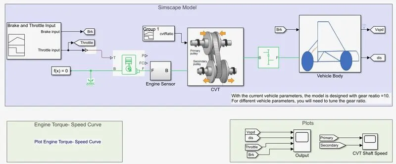
The engine crankshaft is mechanically connected with the continuous variable transmission block (CVT) to drive and adjust the gear transmission and speed of vehicle.

After running the simulation we can observed the results on scope with current vehicle parameter , the model design with Gear Ratio = 10 .

Scope 1 output plots for vehicle , distance, throttle and brake.

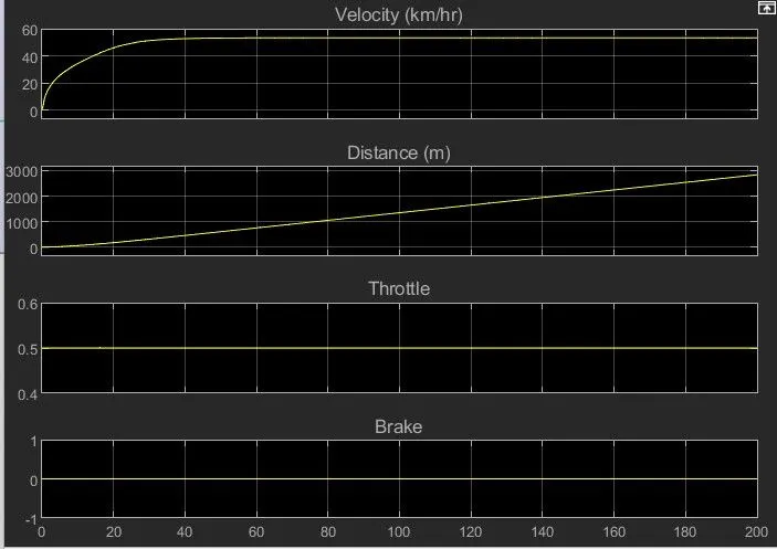
When throttle input is applied then velocity parameter increases quickly with gradually increasing distance. After the distance of about 500 m velocity 52.6 (km/hr) is constant for all time .

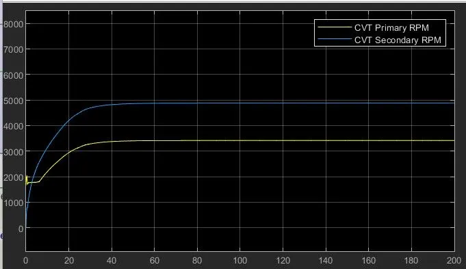
Above plot represents graph for CVT primary and secondary RPM per seconds. After engine starting primary CVT make a spike from 1750 RPM to 2050 RPM then decreases to 1700 RPM and then starts increasing upto 3414 Rpm and then is it constant from 60 sec. But in case of secondary CVT it starts increasing gradually from 0 to 4878 Rpm then it is constant with respect to time.

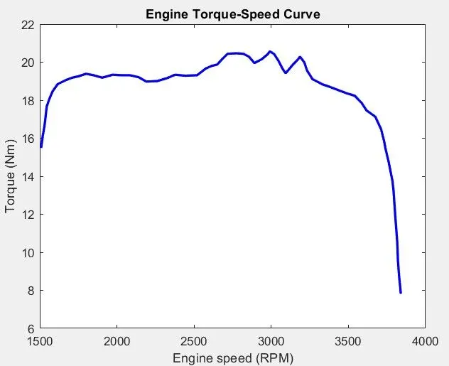
Above plot shows the relation between Speed and Torque . we can observed the actual values of speed and torque in matlab workspace after running the simulation. As workspace interface given below :

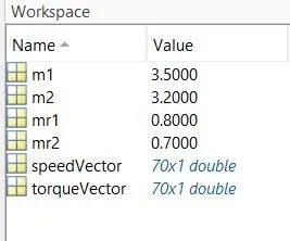
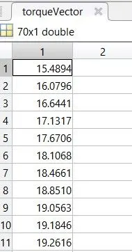
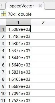
And the actual values for Speed and Torque are as follow :

CASE 2 : BAJA ATV model – Data Extraction (cvtmodel_data)

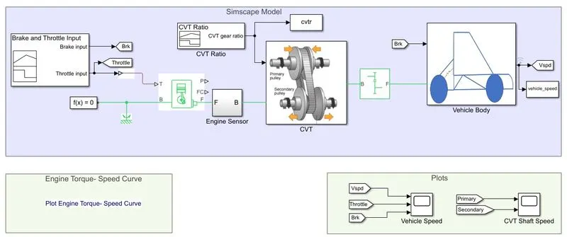
This model is same as our case 1 main model. In this model we are exporting gear ratio data (cvtr) and vehicle speed data (vehicle_speed) to workspace with the help of ‘To Workspace’ block .

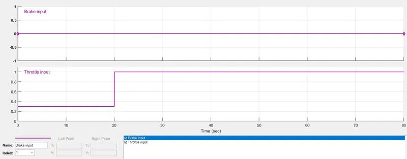
Brake and Throttle input :

Inputs signals are generated with the help of signal builder block. Brake signal is 0 for all the time and throttle signal is 0.3 at stating and then increases to 1 after 20 sec.

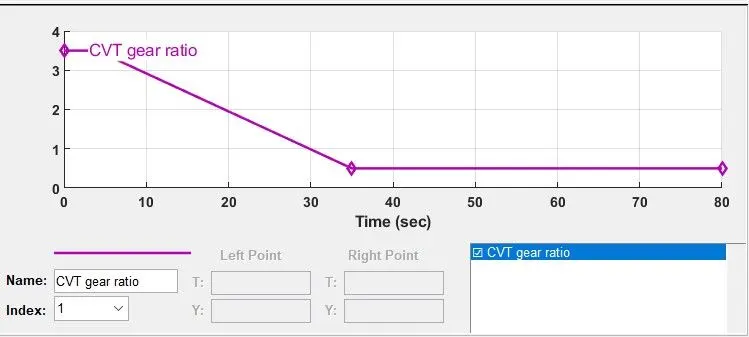
CVT Ratio input :

OUTPUTS :

After applying this input signals we run the simulation and when observed the result the cvt gear ratio and vehicle speed data parameters are stored to matlab workspace.

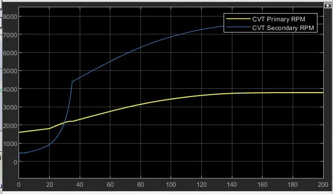
As we can observed on above plot that is the output of CVT shaft , At the staring stage of engine cvt primary shaft speed is grater than cvt secondary shaft speed . after 30 sec CVT secondary shaft speed increases exponentially from 4400 RPM to 7568 RPM .

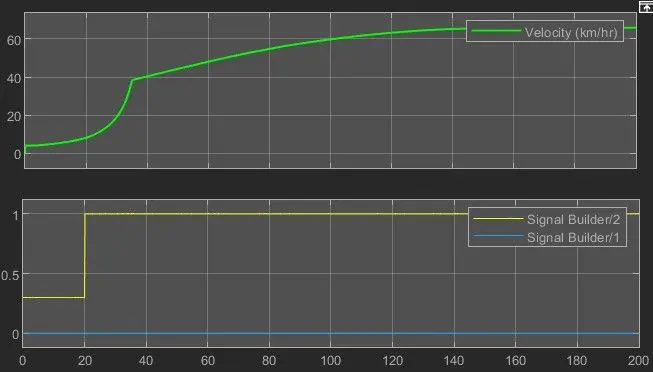
Velocity and CVT secondary speed both output signals having same graph with different values.

Signal 1 is for brake input and signal 2 is throttle signal same as main model. Brake signal is 0 for all time and throttle signal starts from 0.3 and increases after 20 sec and then signal at 1 for all time for this input velocity parameter output appear from 4.04 km/hr then increases gradually.

CASE 3 : BAJA ATV model – With Dashboard (cvtmodel_dashboard)

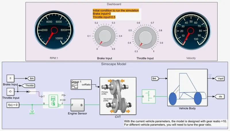
In this model we can apply input signal and observed the output values at dashboard. Blocks used in dashboard are :

Circular Gauge :-

The Circular Gauge block displays the value of the connected signal on a circular gauge that you can design to look like a gauge in a real system. The Circular Gauge block displays the instantaneous value of the connected signal throughout simulation. This block is used to observed the output parameter values of vehicle speed and velocity.

Circular gauge range for vehicle speed parameter is from 0 to 10000 RPM and for velocity it is from 0 to 100 km/hr

Knob :-

The Knob block tunes the value of the connected block parameter during simulation. This block is used to apply the brake and throttle signal to ATV engine. Knob input range for brake signal is from 0 to 0.5 and for throttle signal it is from 0.3 to 1.

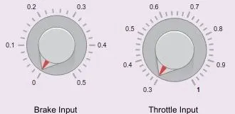
At initial condition to run the simulation brake signal knob is at 0 position and throttle signal knob is at 0.3 .

INPUT AND OUTPUT :

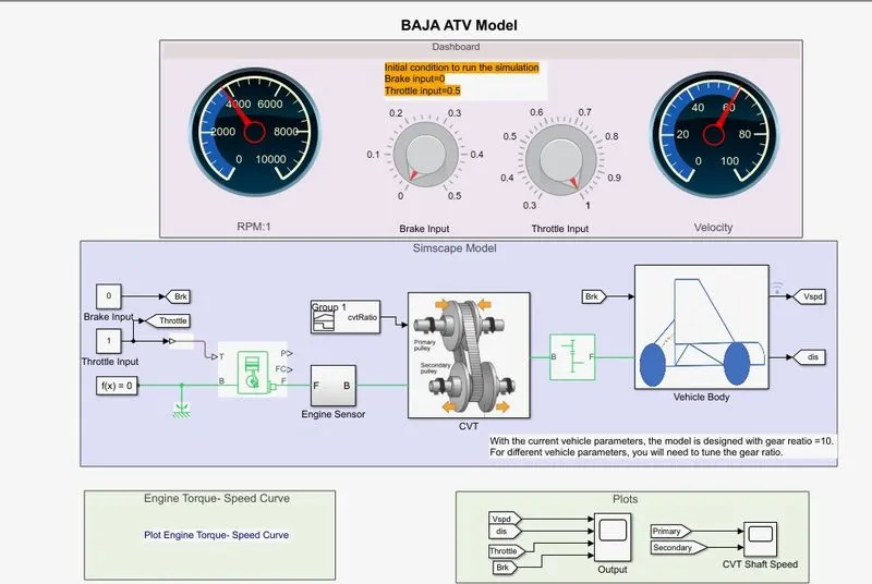
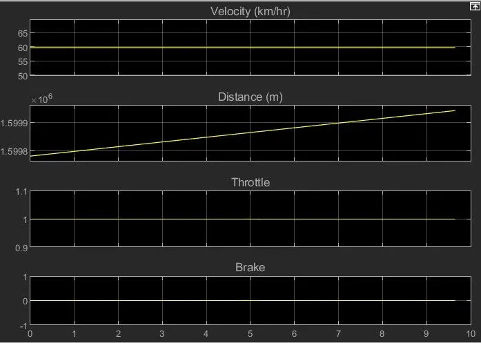
After applying input signals using dashboard knob for brake is 0 and throttle is 0.3. then run the simulation and observed the output values on dashboard . for the distance of 1.59 m vehicle speed is 3810 RPM and velocity is at 60 km/hr .

Brake , Throttle, Distance and Velocity output plot :

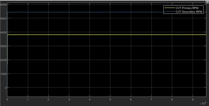
CVT shaft speed plot :

CVT primary shaft speed is 3810 RPM and secondary shaft speed is 5444 RPM .

Engine torque speed curve is same as main model.

CASE 3 : BAJA ATV model – Mapped Lookup Table Without Dashboard (cvtmodel_mapped)

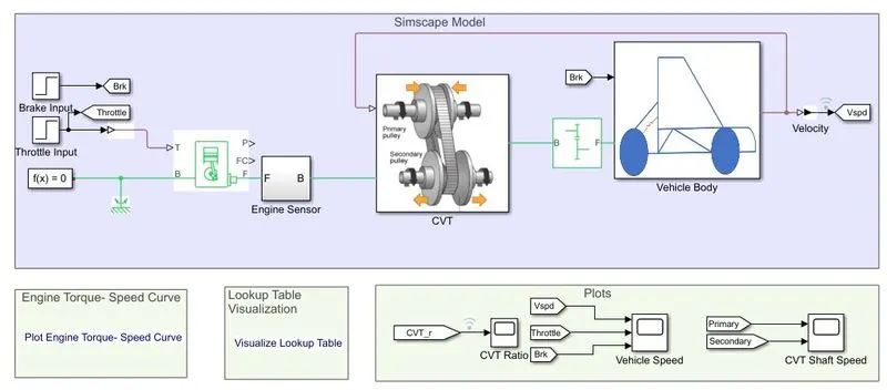
The overall model is same as main model of ATV only the difference in this model is input signal for CVT ratio is change to PS Lookup table block instead of signal builder. Inputs for brake and throttle signals are same as main model i.e. CASE 1

PS Lookup Table :

A lookup table block uses am array of data to map input values to output values, approximating a mathematical function. This block represents a physical signal converter whose input-output relationship is specified by a lookup table. The table grid must be in strictly ascending or strictly descending order, but the spacing can be nonuniform.

CVT SUBSYSTEM WITH 1- D LOOKUP :

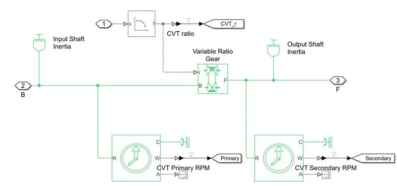
Array of data is save to matlab workspace while running the simulation, data values for lookup table are from 3.5 to 0.5 as we can observed on the plot below :

CVT Ratio Vs Vehicle Speed Output Plot:

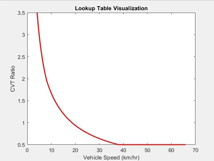
Vehicle speed is directly proportional to CVT ratio of ATV , as speed increases CVT ratio also increases and vise versa.

Output parameters values for CVT shaft speed , Throttle , Brake and engine torque curve are similar to CASE 2 model.

CASE 5 : BAJA AVT model – Mapped Lookup Table with Dashboard ( cvtmodel_dashboard_mapped)

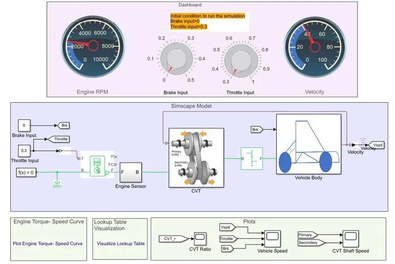
In this model initial condition to run the Simulink input is applied with the help of dashboard knob for brake = 0 and throttle = 0.3 .

Output at initial condition :

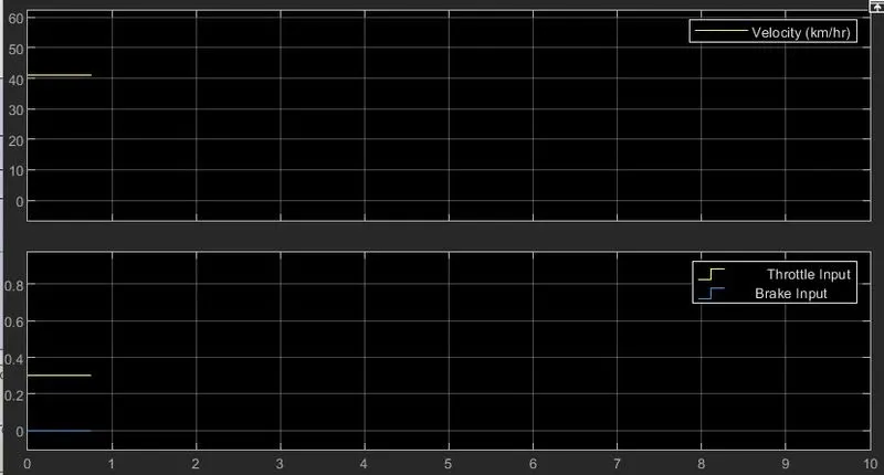
Velocity output value at initial condition is from 0 to 41.93 km/hr and further maintain the level. brake output is 0 and throttle output is 0.309.

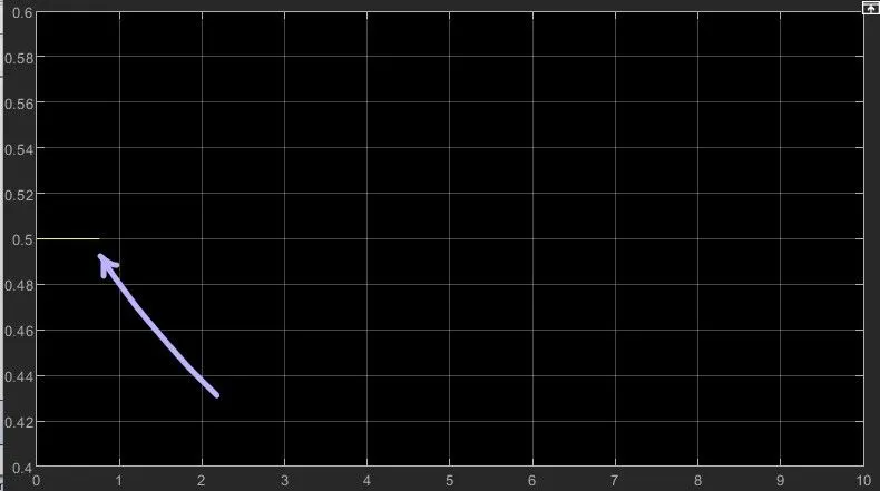
CVT Ratio At Initial Condition : Output for CVT Ratio at initial condition is 0.5

CVT Shaft Speed at Initial :

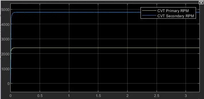
CVT Shaft speed increases quickly in less than a sec. CVT secondary shaft speed is increases from 0 to 4792.63 RPM and then 4794.61 RPM for all time. Primary shaft speed increases from 0 to 2190 RPM the decreases below 2174 RPM again starts increasing to 2396.47 Rpm and then at 2397.3 Rpm for all time.

To observed output at different conditions we changed the input parameters.

Now the brake signal = 0 and Throttle = 0.6.

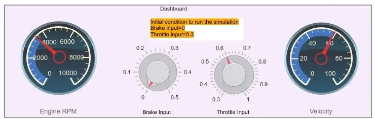
At this condition engine speed and velocity values are changed but, remaining all parameter values are same as at the initial condition.

When throttle is at 0.6 the velocity output increases upto 58.5 km/hr and then 58.87 km/hr for all time.

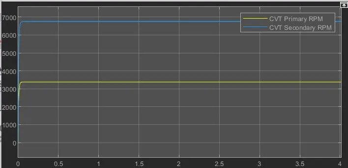
Then CVT shaft speed also varies . CVT primary shaft speed is increases to 3376.125 RPM and same for all the time and CVT secondary shaft speed increase from 0 to 6752.245 RPM and then 6752.25 RPM for all time.

CONCLUSION :

Thus we have successfully studied and analysed all the 5 cases for BAJA ATV Simulink model and recorded the outputs for vehicle speed , velocity , CVT ratio and CVT shaft rpm with respect to variation in input throttle and brake.

REFERENCE :

MATLAB Help

MATHWORKS

https://www.mathworks.com/matlabcentral/fileexchange/70576-baja-all-terrain-vehicle-atv-model