Project
Continuously Variable Transmission (CVT) BAJA All-Terrain Vehicle (ATV)
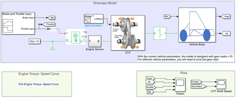
A continuously variable transmission (CVT) is an automatic transmission that can change seamlessly through a continuous range of gear ratios.
This contrasts with other transmissions that provide a limited number of gear ratios in fixed steps. The flexibility of a CVT with suitable control may
allow the engine to operate at a constant RPM while the vehicle moves at varying speeds.
In the BAJA model, we are going to define the gear ratio, and record the response in the effect/variation of the vehicle's main parameters like the vehicle velocity,
and the RPM of the engine by changing the throttle or brake input parameters.
Before going into the model have a look at the important blocks used in this BAJA model.
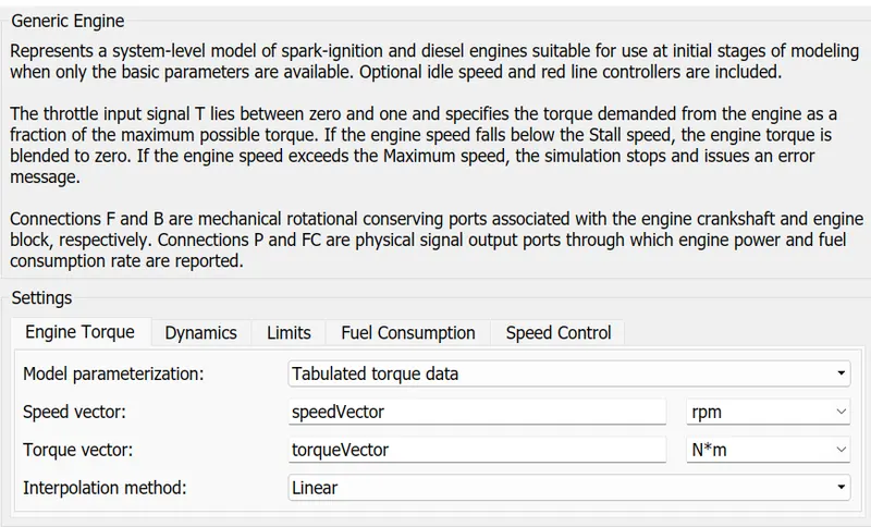
The Generic Engine block represents a general internal combustion engine. This block is a suitable generic engine for spark-ignition and diesel.
Speed-power and speed-torque parameterizations are provided. A throttle physical signal input specifies the normalized engine torque.
The Ideal Rotational Motion Sensor block represents an ideal mechanical rotational motion sensor, that is, a device that converts a variable
measured between two mechanical rotational nodes into a control signal proportional to angular velocity or angle.
The Simple Gear block represents a gearbox that constrains the connected driveline axes of the base gear, B, and the follower gear, F,
to co-rotate with a fixed ratio that you specify.
A continuously variable transmission (CVT) is an automatic transmission that can change seamlessly through a continuous range of gear ratios.
This contrasts with other transmissions that provide a limited number of gear ratios in fixed steps. The flexibility of a CVT with suitable control may
allow the engine to operate at a constant RPM while the vehicle moves at varying speeds.
The Variable Ratio Transmission block represents a gearbox that dynamically transfers motion and torque between the two connected
driveshaft axes, the base, and the follower.
The Inertia block represents an ideal mechanical translational inertia that is described with the following equation:
T=J*dω/dt where:i) T is inertia torque, ii) J is inertia. iii) ω is the angular velocity, and iv) t is time.
The Tire (Magic Formula) block models a tire with longitudinal behavior given by the Magic Formula, an empirical equation based on four fitting
coefficients. The block can model tire dynamics under constant or variable pavement conditions.
The Vehicle Body block represents a two-axle vehicle body in longitudinal motion. The vehicle can have the same or a different number of
wheels on each axle.
The Double-Shoe Brake block represents a frictional brake with two pivoted rigid shoes that press against a rotating drum to produce a braking action.
The Circular Gauge block displays the value of the connected signal on a circular gauge that you can design to look like a gauge in a real system.
The Knob block is used to tune the value of a variable or block parameter during simulation.
The agenda of this Vehicle Modelling is to define the gear ratio, find out the effect of parameter variation, and Incorporate CVT data into the model
The major component of a BAJA ATV model is a.Vehicle body, b. Suspension, c.Tire, and d.Engine, and e.Continuously Variable Transmission (CVT)
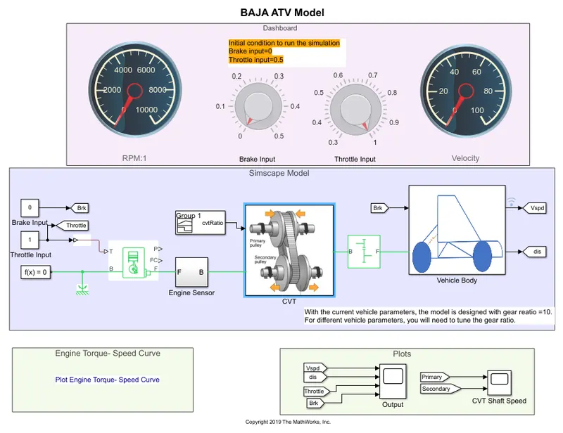
Modeling of Different Components:
Tire Modelling:
Just default values are taken in the block, if we have data for the specific tire we can feed in and try.
Engine block:
When we click on the generic engine it asks for a few values like speed vector and torque vector.
Simulator Data Inspector is used to compare the vehicle speed at different masses (Data inspector can run multiple simulations)
To get the result we need to lock the signals, Example if we want to measure the velocity in the model initially, we have to lock the signal as mentioned in the Model (Vspd)
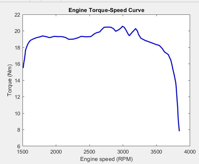
If we suppose the data is in the form of an image (Engine speed (X-axis) vs Torque (Y-axis)), Using the Grabit file exchange method we can extract the data points and these data points we can feed into the generic engine.
The data which u feed is given in the model as a link as Plot (Engine Torque – Speed Curve)
The next component is CVT. It consists of
- Primary pulley, 2. Variator, 3. Secondary pulley, and 4. Belt
The variator which is connected to the primary pulley when it goes outward the variator of the secondary pulley move inward such that the radius of the secondary pulley is more than the radius of the primary pulley.
CVT Ratio:
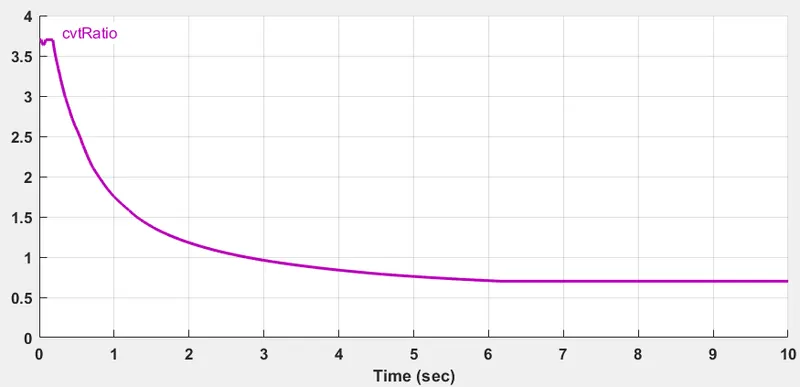
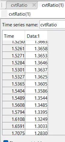
Rp < Rs (That will lead to speed reduction)
On the other hand, when the variator of the primary pulley moves inward the variator of the secondary pulley will move outward.
Rp > Rs (will lead to overdrive)
The BAJA ATV model has various components like an engine, CVT block, and vehicle body.
By varying the parameters on the BAJA All-Terrain Vehicle (ATV) Model the following two tests were conducted and the results are analyzed.
A.Break performance test:
B.CVT characteristic analysis: (Vehicle weight and CVT ratio)
A.Break performance test:
1. We are giving input as Brake input 0 and throttle input as 1 and after 100sec. Brake input 1 and throttle input as 0 as shown below.
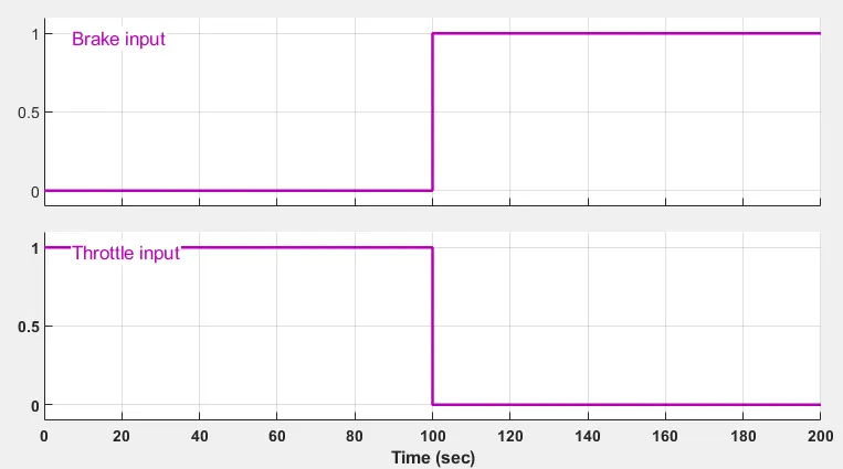
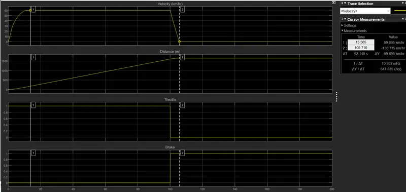
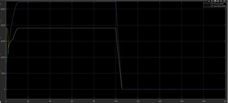
From the result, it can be seen that if the throttle increases the velocity also increases after 13.565 sec. it reaches maximum velocity (59.685km/hr).
and after the break input as 1, the time taken to reach zero velocity is 5.7sec. (Ref. file name in the attachment: 1.CVToutput.fig & 1.Velocity.fig)
2. We are giving input as Brake input 0 and throttle input is initially 0.5 then gradually raised to 1.0 at 100sec. then after 0 as shown below.
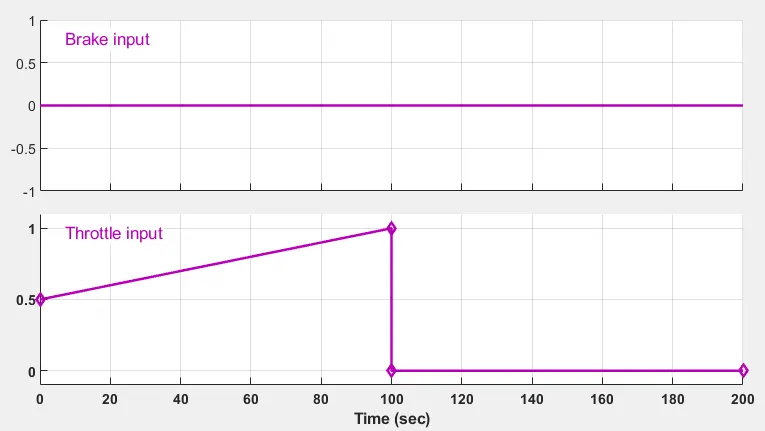
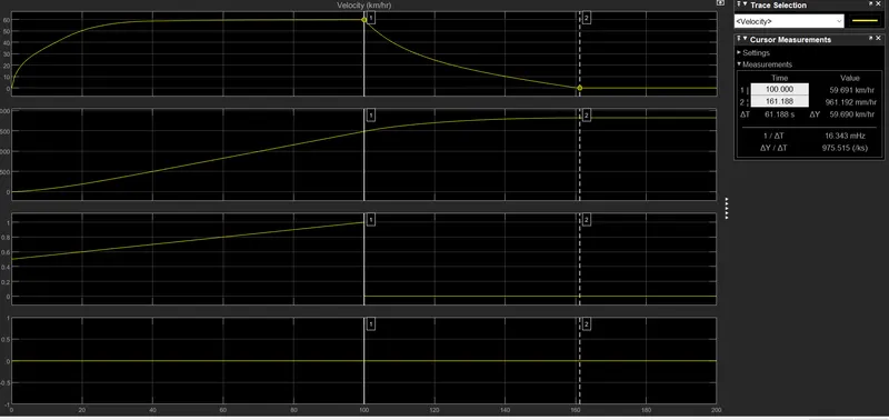
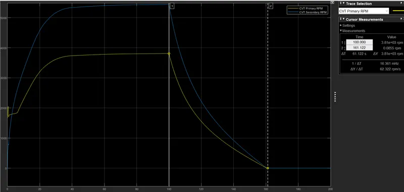
From the result, it can be seen that if the throttle increases the velocity also increases as per throttle opening and it reaches maximum velocity (59.685km/hr).
and after100th sec. the break input as 1, the time taken to reach zero velocity is 61.7sec. (Ref. file name in the attachment: 2.CVToutput.fig & 2.Velocity.fig)
B.CVT characteristic analysis: (Vehicle weight and CVT ratio)
The nature of the curve of vehicle velocity and the CVT of the secondary pulley is the almost same reason being it is connected to the rear wheel.
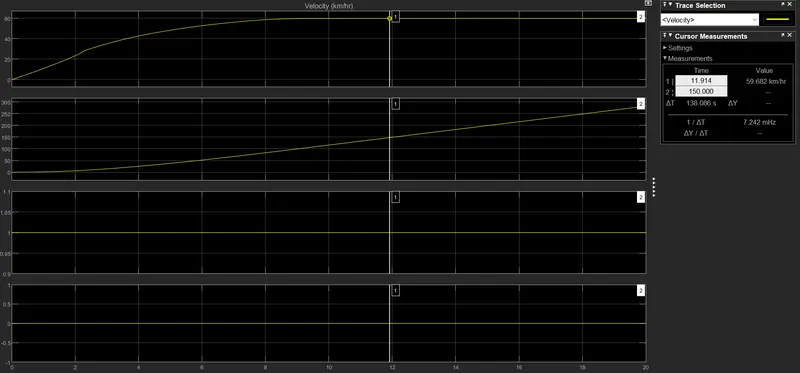
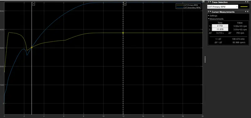
i) Analysis for the vehicle body mass 200 kg
(for our easy understanding, We are giving the Break Input = 0 & Throttle = 1 and Simulation stop time: 20 seconds)
As shown in the below graph the vehicle takes 12 seconds to reach maximum velocity (59.685 km/hr) also the CVT Primary RPM and CVT Secondary RPM reaches the maximum,
The meeting point of CVT primary RPM and CVT secondary RPM is 2.75Sec. Beyond 2.75 seconds CVT secondary RPM increases than the CVT primary RPM.
(Ref. file name in the attachment: Velocity200KG.fig & CVT200KG.fig)
ii) Analysis for the vehicle body mass 500 kg
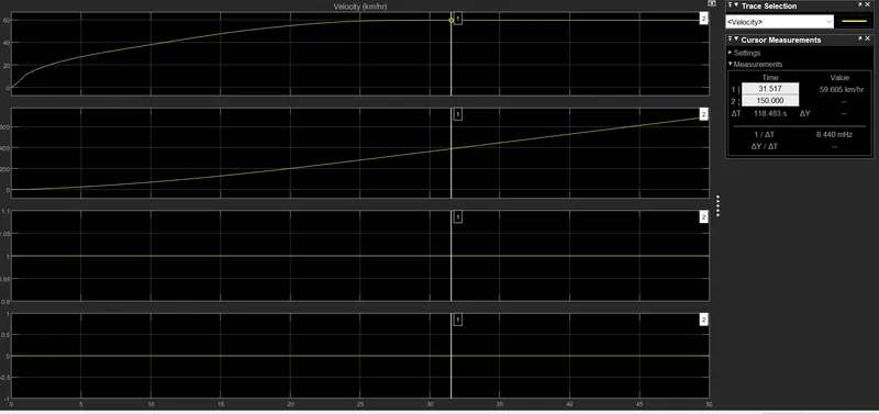
(for our easy understanding, We are giving the Break Input = 0 & Throttle = 1 and Simulation stop time: 50 seconds)
As shown in the below graph the vehicle takes 31.5 seconds to reach maximum velocity (59.605 km/hr) also the CVT Primary RPM and CVT Secondary RPM reaches the maximum,
The meeting point of CVT primary RPM and CVT secondary RPM is 2.75Sec. Beyond 2.75 seconds CVT secondary RPM increases than the CVT primary RPM.
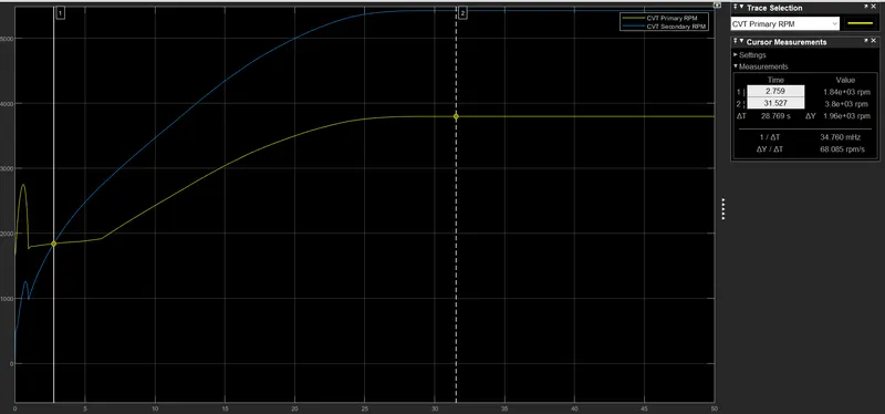
From the above analysis, it can be inferred that irrespective of the vehicle body mass the meeting point of CVT primary RPM and CVT secondary RPM is the same (2.75 Sec)
whereas the time taken to reach the maximum velocity for the vehicle mass is 200 kg (12 Sec) is less compared to the vehicle mass 500 kg is more (31.5 Sec).
(Ref. file name in the attachment: Velocity500KG.fig & CVT500KG.fig)