Project
- BAJA All-Terrain Vehicle (ATV) Model :
- MODEL:-
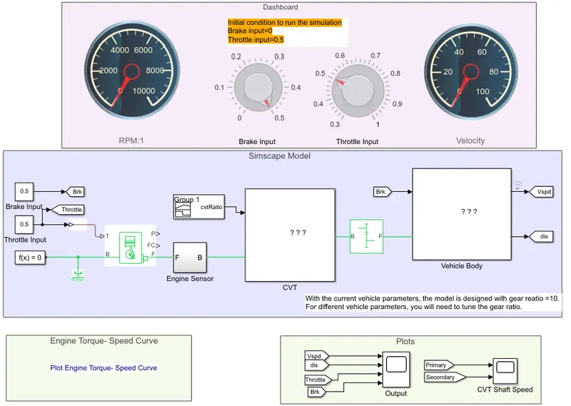
- 1ST CASE( WHEN BRAKE INPUT=0 AND TROTTLE INPUT=0.5):-
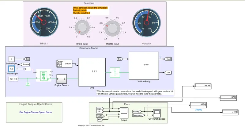
VEHICLE AND CVT GRAPH:
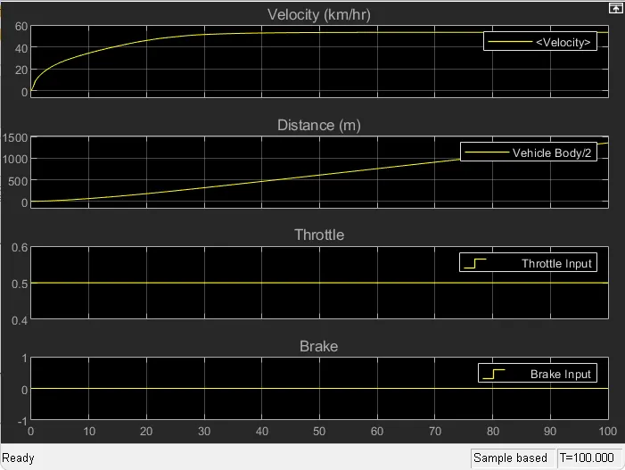
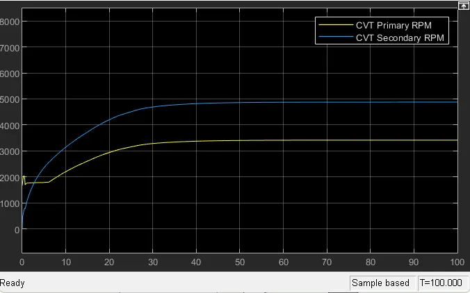
RESULT:- In CVT Primary speed 3415 RPM and Secondary speed 4878 RPM. Then Vehicle speed 53.53 km/hr and Distance 1352 m.
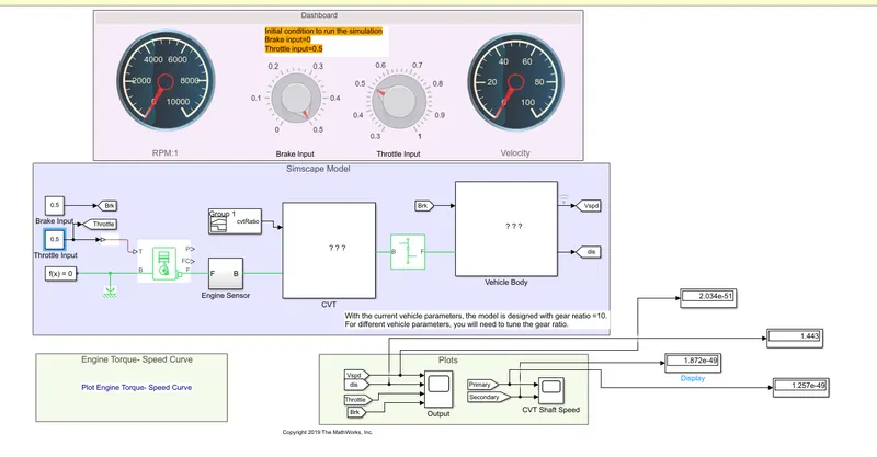
- 2ND CASE(WHEN BRAKE INPUT=0.5 AND TROTTLE INPUT=0.5):-
VEHICLE AND CVT GRAPH:
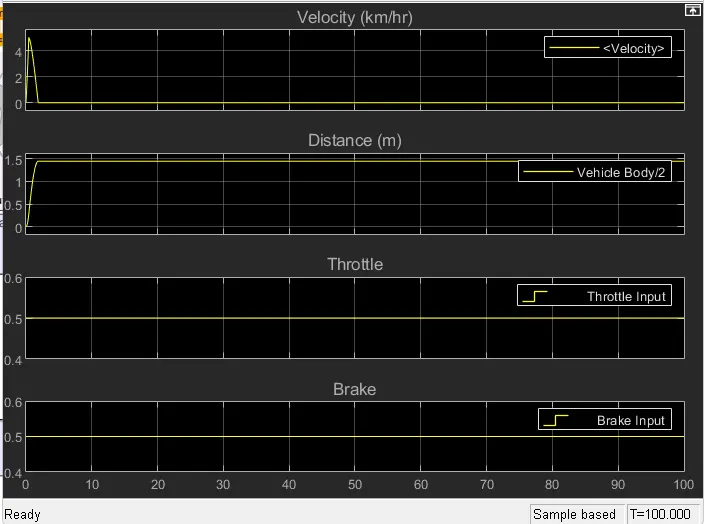
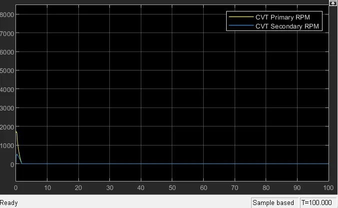
RESULT:- In CVT primary speed 1.257e-49 RPM and Secondary speed 1.872e-49 RPM. Then vehicle speed 2.034e-51 Km/hr and distance 1.443m.
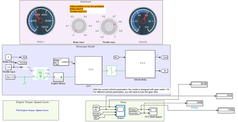
- 3RD CASE(WHEN BRAKE INPUT=0 AND TROTTLE INPUT=O.8):-
VEHICLE AND CVT GRAPH:
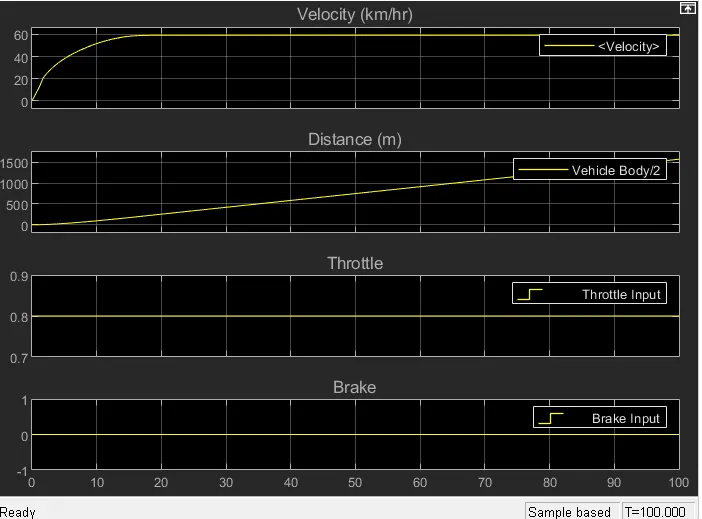
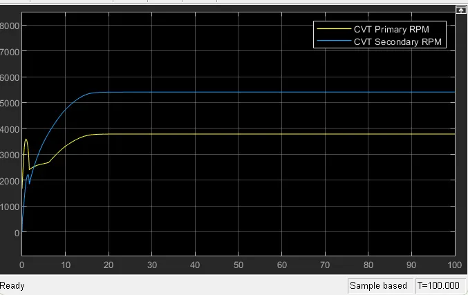
RESULT:- In CVT Primary speed 3784 RPM and Secondary speed 5406 RPM. Then Vehicle speed 59.29 km/hr and Distance 1572 m.
- BLOCK CONNECTION WITH VEHICLE BODY DIAGRAM:-
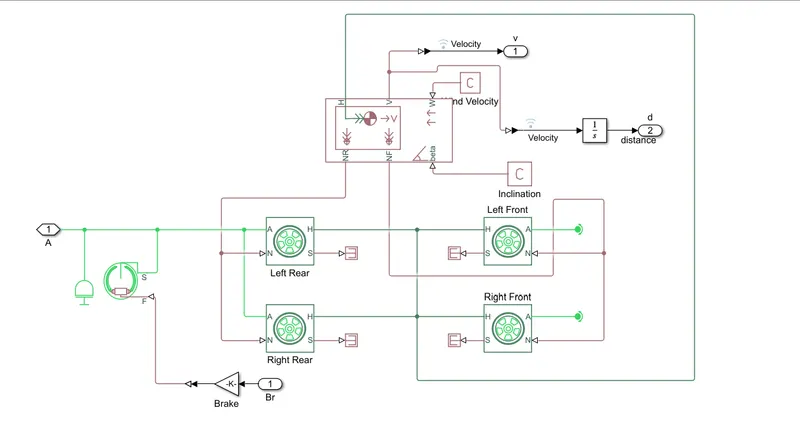
- Block used connection with vehicle body:-
The Inertia block represents an ideal mechanical translational inertia that is described with the following equation:
T=Jdωdt
where:
-
T is inertia torque.
-
J is inertia.
-
ω is angular velocity.
-
t is time.
By default, the block has one mechanical translational conserving port. The block positive direction is from its port to the reference point. This means that the inertia torque is positive if inertia is accelerated in the positive direction.
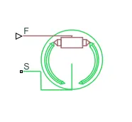
2. Double shoe brake:-
The Double-Shoe Brake block represents a frictional brake with two pivoted rigid shoes that press against a rotating drum to produce a braking action. The rigid shoes sit inside or outside the rotating drum in a diametrically opposed configuration. A positive actuating force causes the rigid shoes to press against the rotating drum. Viscous and contact friction between the drum and the rigid shoe surfaces cause the rotating drum to decelerate.
Double-shoe brakes provide high braking torque with small actuator deflections in applications that include motor vehicles and some heavy machinery. The model employs a simple parameterization with readily accessible brake geometry and friction parameters.
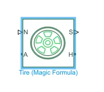
3. Tire(Magic Formula):-
The Tire (Magic Formula) block models a tire with longitudinal behavior given by the Magic Formula [1], an empirical equation based on four fitting coefficients. The block can model tire dynamics under constant or variable pavement conditions.
The longitudinal direction of the tire is the same as its direction of motion as it rolls on pavement. This block is a structural component based on the Tire-Road Interaction (Magic Formula) block.
To increase the fidelity of the tire model, you can specify properties such as tire compliance, inertia, and rolling resistance. However, these properties increase the complexity of the tire model and can slow down simulation. Consider ignoring tire compliance and inertia if simulating the model in real time or if preparing the model for hardware-in-the-loop (HIL) simulation.
Model:-
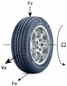
The Tire (Magic Formula) block models the tire as a rigid wheel-tire combination in contact with the road and subject to slip. When torque is applied to the wheel axle, the tire pushes on the ground (while subject to contact friction) and transfers the resulting reaction as a force back on the wheel. This action pushes the wheel forward or backward. If you include the optional tire compliance, the tire also flexibly deforms under load.
The figure shows the forces acting on the tire. The table defines the tire model variables.
4. Vehicle body:-
The Vehicle Body block represents a two-axle vehicle body in longitudinal motion. The vehicle can have the same or a different number of wheels on each axle. For example, two wheels on the front axle and one wheel on the rear axle. The vehicle wheels are assumed identical in size. The vehicle can also have a center of gravity (CG) that is at or below the plane of travel.
The block accounts for body mass, aerodynamic drag, road incline, and weight distribution between axles due to acceleration and road profile. Optionally include pitch and suspension dynamics. The vehicle does not move vertically relative to the ground.
The block has an option to include an externally-defined mass and an externally-defined inertia. The mass, inertia, and center of gravity of the vehicle body can vary over the course of simulation in response to system changes.
MODEL:
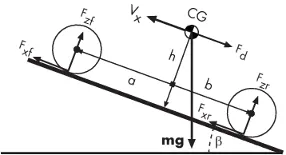
he vehicle axles are parallel and form a plane. The longitudinal, x, direction lies in this plane and perpendicular to the axles. If the vehicle is traveling on an incline slope, β, the normal, z, direction is not parallel to gravity but is always perpendicular to the axle-longitudinal plane.
This figure and table define the vehicle motion model variables.
Vehicle Dynamics and Motion
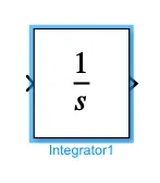
5. Integrator:-
The Integrator block outputs the value of the integral of its input signal with respect to time.
Simulink® treats the Integrator block as a dynamic system with one state. The block dynamics are given by:
{˙x(t)y(t)=u(t)=x(t) x(t0)=x0
where:
-
u is the block input.
-
y is the block output.
-
x is the block state.
-
x0 is the initial condition of x.
6.Gain:-
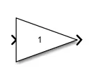
The Gain block multiplies the input by a constant value (gain). The input and the gain can each be a scalar, vector, or matrix.
You specify the value of gain in the Gain parameter. The Multiplication parameter lets you specify element-wise or matrix multiplication. For matrix multiplication, this parameter also lets you indicate the order of the multiplicands.
Gain is converted from doubles to the data type specified in the block mask offline using round-to-nearest and saturation. The input and gain are then multiplied, and the result is converted to the output data type using the specified rounding and overflow modes.
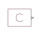
7.PS Constant:-The PS Constant block generates a physical signal of a constant value. You specify the value and unit of the signal as the Constant parameter.
8. PS Terminator:-
Use the PS Terminator block to cap physical signal output ports that do not connect to other blocks.
Unlike conserving ports in physical modeling, or Simulink® output ports, unconnected physical signal output ports do not generate warnings. However, you can use a PS Terminator block for clarity, to indicate that the signal was not inadvertently left unconnected.
9. Rotational free end:-
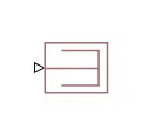
The Rotational Free End block represents a mechanical rotational port that rotates freely, without torque.
You can use this block to terminate mechanical rotational ports on other blocks that you want to leave unconnected. This is not necessary because if you leave a conserving port unconnected, the physical network sets all the Through variables at that port to 0. However, terminator blocks improve diagram readability.
You can also use this block to set the initial rotational velocity at a node.
10. Inport:-Inport blocks link signals from outside a system into the system.
11. Outport:- Outport blocks link signals from a system to a destination outside of the system. They can connect signals flowing from a subsystem to other parts of the model. They can also supply external outputs at the top level of a model hierarchy.
12. Simulink-ps converter:- The Simulink-PS Converter block converts the input Simulink signal into a physical signal. Use this block to connect Simulink sources or other Simulink blocks to the inputs of a Simscape™ physical network.
13. PS-Simulink converter:- The Simulink-PS Converter block converts the input Simulink signal into a physical signal. Use this block to connect Simulink sources or other Simulink blocks to the inputs of a Simscape™ physical network.
