Project

Q. Carry out a system-level simulation of an all-terrain vehicle.

Download the model from the given link:

https://www.mathworks.com/matlabcentral/fileexchange/70576-baja-all-terrain-vehicle-atv-model

Prepare a technical report explaining the model properties & comments on the results.

Ans.

1. CVT MODEL

• To understand this problem first we understand that what is ATV model?
• ATV(all terrain vehicle) is low weight vehicle which is used in off road activities mostly ans aslo on road activities. Below image is provide.

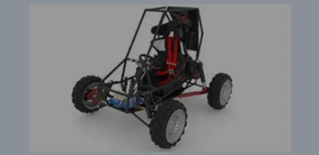
• This type of vehicle that travels on low pressure tires, along with handlebars for steering control.

Block used in this model :-

• Signal builder :- Based on our requirement we can build the signal in terms of continue value.
• Generic engine:- This block is use as initial engine means basic level understanding of engine, here we used as ATV’s engine.
• Simple gear:- To provide fix gear ratio between to gear for speed reduce or increase.
• PS terminator :- To close the open physical port because some open physical port may generate error in diagnostic window.
• Ideal mechanical rotational sensor:- To show rotational speed of shaft.
• Shaft inertia:- Ideal mechanical rotational inertia which is provide tendency to resist changes at input side and output side.
• Variable ratio transmission:- Variable gear ratio box change in continue manner with consider friction loss, transmission loss and viscous loss.
• Tire(magic formula):- Used as tire.
• Vehicle body:- Consider as vehicle body.
• Double shoes brake:- To exert friction torque in wheel shaft.
• Rotational free end:- To free rotate wheel without torque.
• Scope:- See the result in term of graphical representation.
• Mechanical rotational reference:- Frame or ground to rigidity fix of model.
• Solver configuration:- Define solver configuration of model.
• Constant:- Give constant value.
• PS converter:- Physical signal to Simulink signal convertor.

Below image provide of BAJA ATV Model

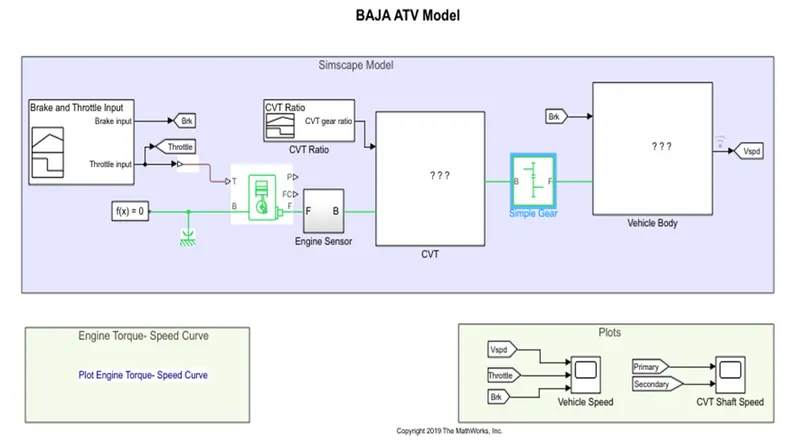
• For generic engine port T connect with throttle input(accelerrator) which is get by signal builder.
• In signal builder two signal is generate first is throttle for engine input and second brake for tire. Generate signal graph is below shows.

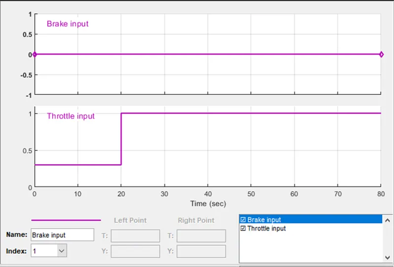
• In this graph we can see that brake torque is constant and throttle input or we can say accelerator change after 20sec.
• Generic engine port B is connected with reference and solver configuration and port P and FC is power output and fuel consumption respectively but here not used.
• Port F is mechanical rotational conserving port associated with the engine crankshaft.
• That crankshaft power and RMP go to variable gear transmission ratio and based on that ratio we get output RPM.
• After variable gear transmission connect to the simple gear ratio to fix type of gear ratio generate which connect to direct with tire.
• In CVT subsystem we change the gear ratio continue with help of signal builder connect with variable gear ratio block.
• CVT subsystem image is below provide.

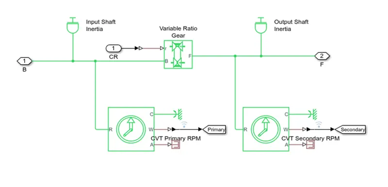
• In above image we see that input and output shaft inertia is provide to tendency to resist changes it can positive or negative.
• In model image we see the vehicle body subsystem.
• In this subsystem we put vehicle body and tire of BAJA ATV. This subsystem image below provide.

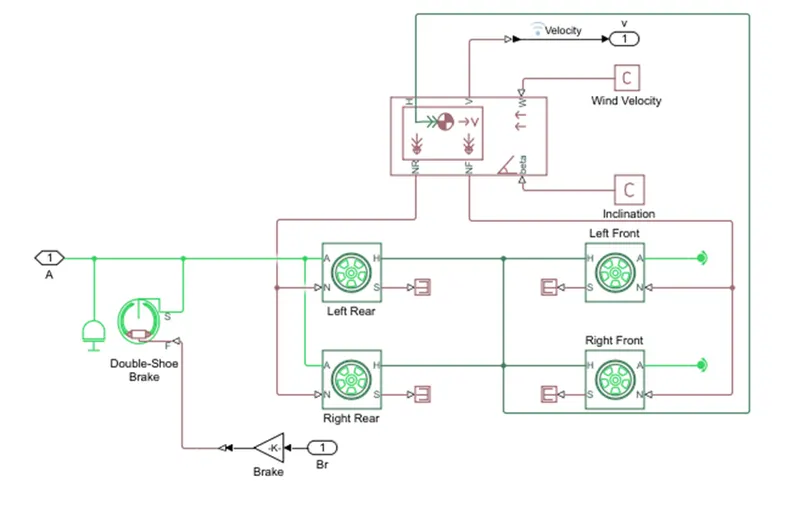
• In this image we can see that vehicle block which represent the two axle body in longitude motion or we can see horizontal body of vehicle with two axle.
• This block provide weight, weight distribution between two axles due to motion in road profile and road inclination means angle between body and road, aerodynamic consideration.
• Their ports H provide horizontal motion of body, V for vehicle velocity, NR and NF for normal force on tire rear and front respectively, B port for inclination of vehicle in road profile, W for headwind speed.
• In this subsystem we can see this tire(magic formula) block used as tire of vehicle. In that block some ports are given A,N,S,H.
• Port A is for conversing of mechanical rotation motion for wheel axles. Port N is provide normal force on tire. Port S is give us to slip of wheel. Port H is for mechanical translational of horizontal motion or thrust for move to tire.
• Here in this subsystem we use brake shoes block which provide resist speed of shaft or axle.

Now we discuss about result of above system.

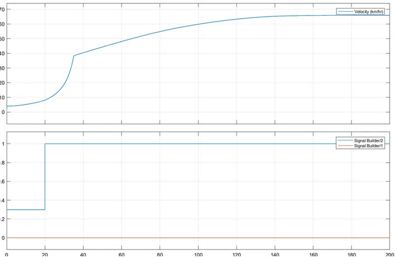
variable speed graph above

• In above graph we can see that velocity Vs time as time increasing of time velocity is increase but velocity is increase because of the throttle value is increase and brake value is constant.
• But in between 0-20 second our velocity is increasing because of achieving throttle value to velocity take some time so velocity increase at constant throttle. After 20 second suddenly throttle value reach 0. 3 to 1 so engine give more RPM to the crankshaft and velocity is increase suddenly as to reach optimize value of velocity at throttle value 1 take some time to velocity so it’s increase in that manner. We understand different case in further report.

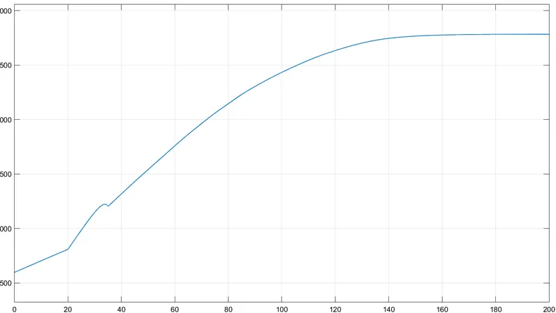
• Engine RMP is depend on the throttle value as we increase the value of throttle engine RPM also increase.
• Here take one case which prove that engine RPM is depend on the throttle value which image provide below.

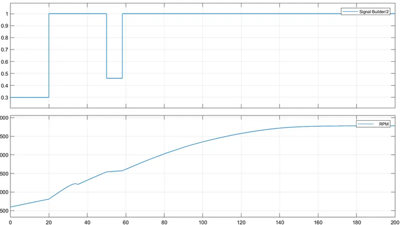
• In above graph when the throttle value decrease at that time also engine RPM is decrease here we see not much decrease in RPM as much throttle because of after that suddenly throttle value increase so we didn’t see much negative falling edge.

• Here take one case which is put some value in brake and see the effect of that and graph of that is provide below.

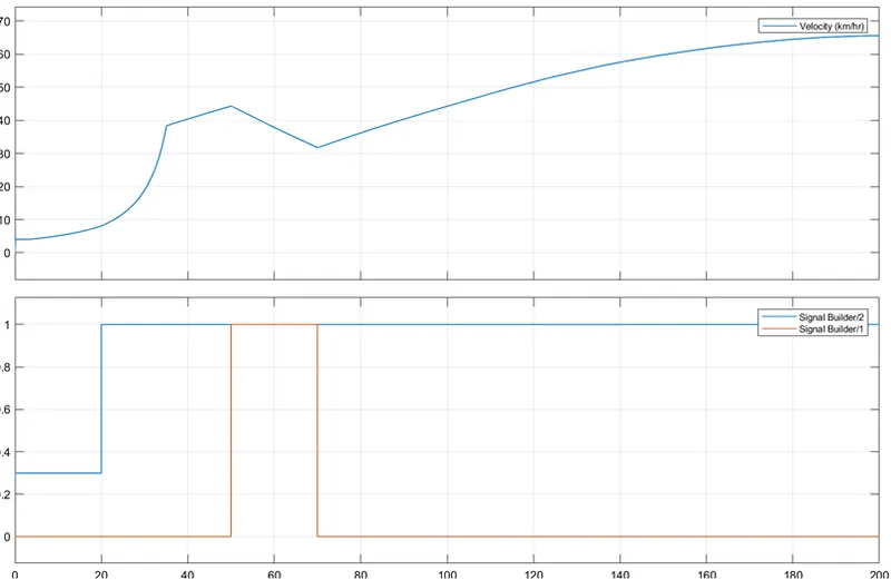
• In above image we can see that if we give some in brake then it’s effect on that velocity here shows this in 50-70 in between hence we prove that the brake block is used to resist that torque in shaft or axles and velocity of tire is decrease that shows in above graph.

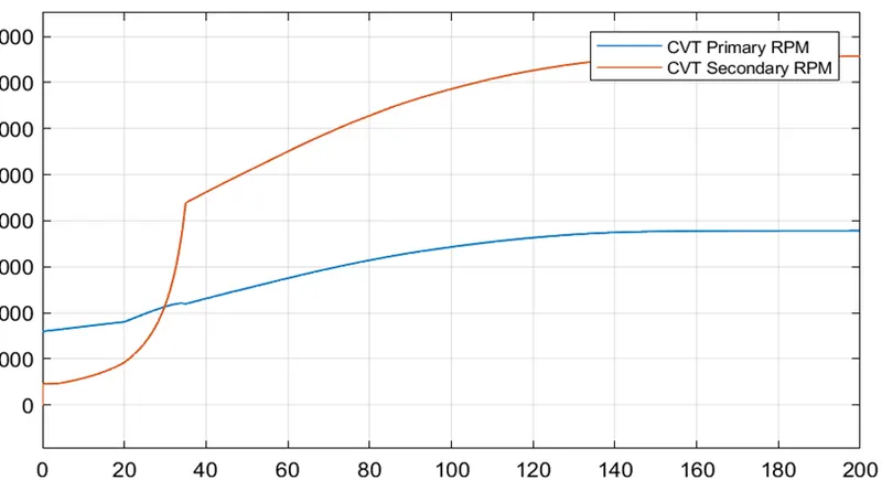
CVT shaft speed graph above

• To understand this graph we require to see the CVT ratio in term of signal builder graph which is given below.

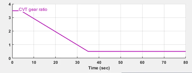
• CVT ratio graph we can see in this graph and observe that when at 5 second our CVT ratio is decreasing with time at that time speed of secondary RPM is increase because of ratio is decreasing.
• At 30 second ratio is 1 at that time our secondary and primary RPM is same or equal after that time at constant ratio both graph slope is same after some time.
• Now it’s time to see all value graphs in one graph with help of data inspector which graph is provide below.

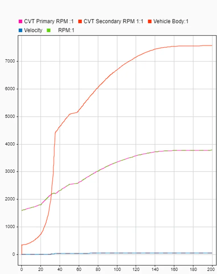
Simulation Data inspector

• Now we discuss about engine torque Vs speed curve which image shows in below.

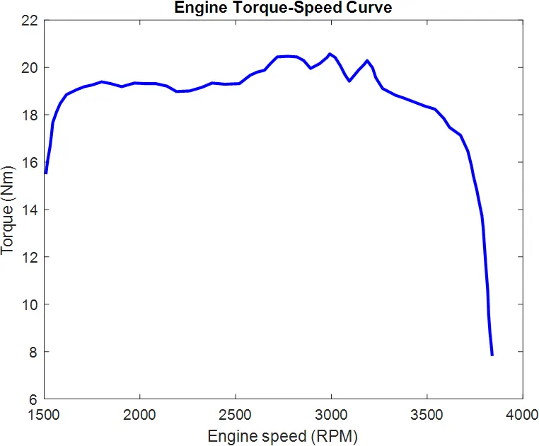
• In this image we can see that in initial time torque is increasing as speed increase after some time speed increase but no more change in torque and after high speed at that time torque is getting decreasing sharply.

2. CVT MODEL DASHBOARD

• In CVT model dashboard same as CVT model but here add some animation block which is help us to visualization speed, engine RPM, brake value and throttle value.
• Other change is like throttle value is also constant is equal to 1 and brake value is same as CVT model is 0.
• Here we also plot graph of distance which is not provide in CVT model.
• For distance we integration of velocity which is provide distance value.

Model image is provide below.

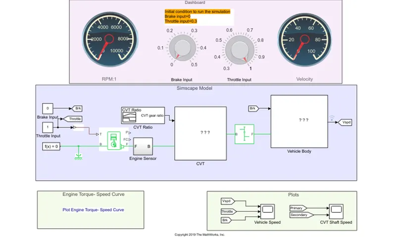
• In above model we can see that with help of dashboard block we can easily see the real time value of engine RPM, velocity of vehicle, brake value and acceleration value.
• Now we discuss about result, as we know that we get same result as CVT model so we are not more discuss on it but here I have to show some graph.

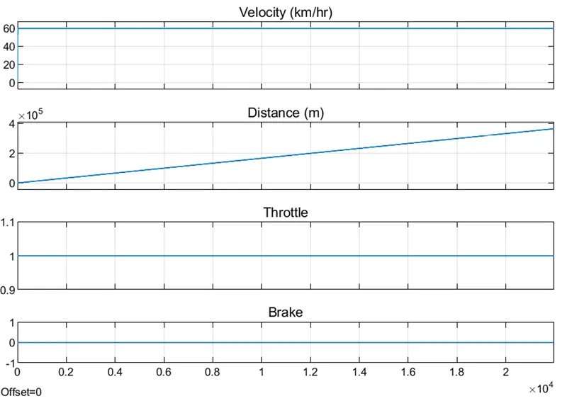
• Here we can see that no more change in value of velocity it’s because of our throttle value is not change through out the run time so here not change velocity value.
• If velocity is decreasing also the out distance value is increasing and if velocity s zero than distance is constant value.
• And velocity is depend on throttle value and brake value.
• CVT shaft speed graph is also same as we above discuss so here not discuss about it.
• Same graph we get in torque Vs speed so here we are not discuss about it.

3. CVT Model_data

• This model same as the CVT model but here we create some variable through model and see the value of that variable.
• Model image is below provide.

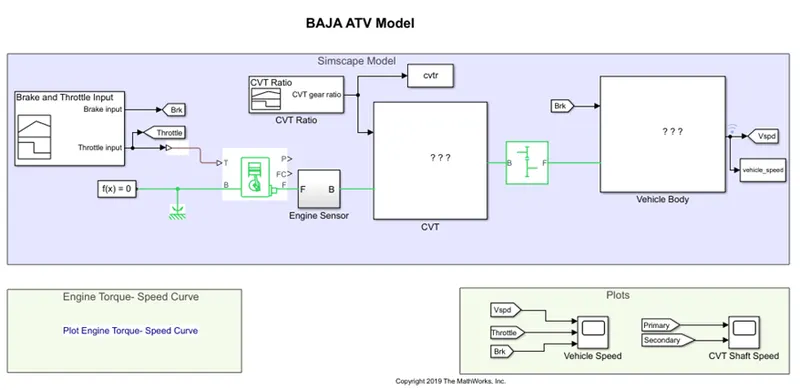
• Here we are created two variable cvtr and vehicle_speed which shows in base workspace and crate by model.
• Before the run model here show image of workspace and after run model show image in that we can see that the variable is add in workspace.

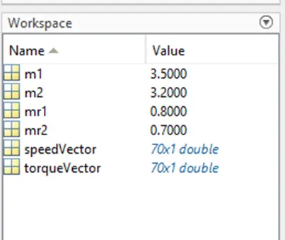
Before run model

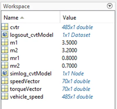
After run model

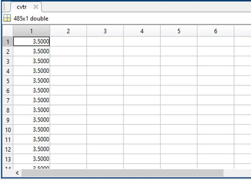
• Cvtr has this data which is store in that variable.

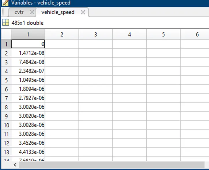
• Vehicle_speed has data which is store in that variable.
• All other result are same so we are not repeat that part.

4. CVT model mapped

Model image is below provide.

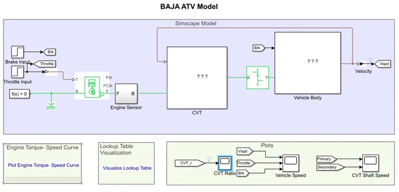
• In that model we can see that CVT ratio is given as feedback loop or close loop as well as data file which is generate CVT ratio with help of look up table.
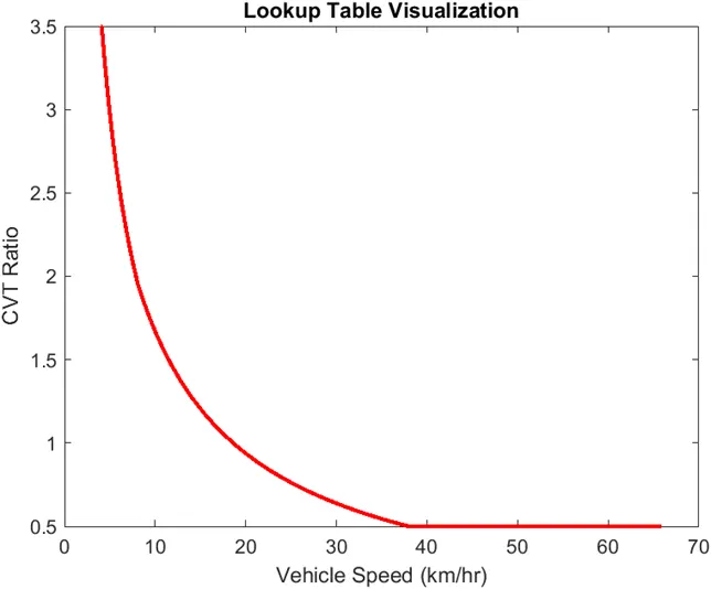
• In this model here we use as same input as above models but in CVT ratio we take look up table and in that look up table we take input as data file which is import in workspace.
• Here all other parameter and value is same so we not discuss about but CVT ratio graph below image is provide.

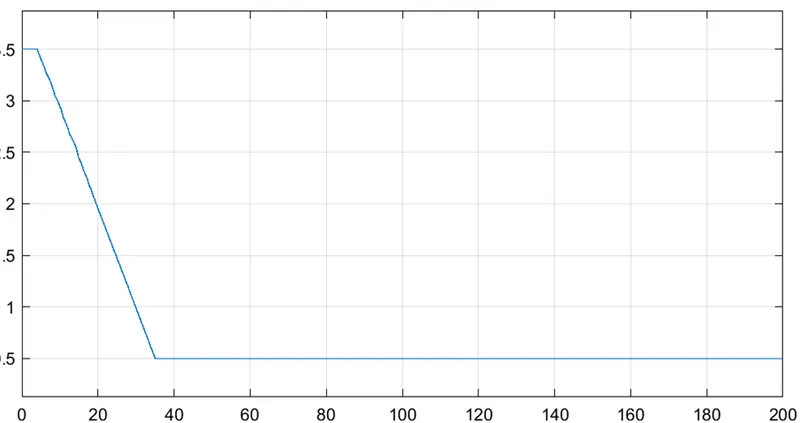
• This same as above we give from signal builder so here we get same value of the primary shaft and secondary shaft RPM graph.
• Here also given look up table visualization figure which is provide below.

5. CVT model dashboard mapped

Model image is provide below.

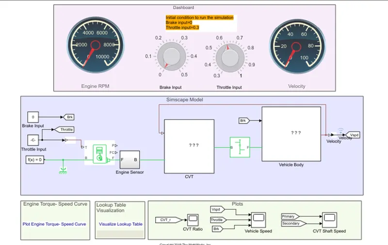
• All block and function are same but for easily see the value for speed and throttle, brake value is see in this dashboard.
• All result are same so we didn’t need to explain result for this model.

CONCLUSION:- we have successfully analysed 4 different models of BAJA AVT with CVT and recoreded output and see the different output graph.