Project

SYSTEM LEVEL SIMULATION OF AN ALL-TERRAIN VEHICLE

AIM

To carry out a system-level simulation of BAJA ATV (All-Terrain Vehicle) and to prepare a detailed technical report explaining the model properties for the following cases:

• Baja ATV model without a dashboard
• Baja ATV model with a dashboard
• Baja ATV model with a look-up table without dashboard
• Baja ATV model with a look-up table and dashboard

THEORY

ALL TERRAIN VEHICLE

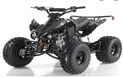
An all-terrain vehicle (ATV) is a motorized off-highway vehicle designed to travel on four low-pressure or non-pneumatic tyres, having a seat designed to be straddled by the operator and handlebars for steering control.As the name implies, it is designed to handle a wider variety of terrain than most other vehicles. Although it is a street-legal vehicle in some countries, it is not street-legal within most states, territories, and provinces of Australia, the United States or Canada.The rider sits on and operates these vehicles like a motorcycle, but the extra wheels give more stability at slower speeds. Although most are equipped with three or four wheels, six-wheel models exist for specialized applications. Multiple-user analogues with side-by-side seating are called utility terrain vehicles (UTVs) or side-by-sides to distinguish the classes of vehicle.

CONTINUOUSLY VARIABLE TRANSMISSION

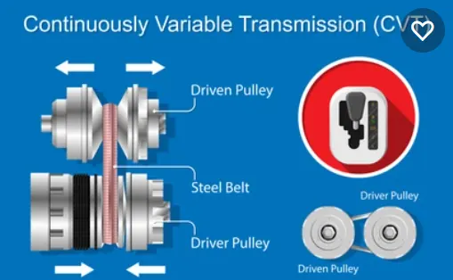
A continuously variable transmission (CVT) is defined as an automatic transmission that can change seamlessly through a continuous range of gear ratios. This contrasts with other transmissions that provide a limited number of gear ratios in fixed steps. The flexibility of a CVT with a suitable control may allow the engine to operate at a constant RPM while the vehicle moves at varying speeds. CVTs are used in automobiles, tractors, motor scooters and earthmoving equipment.The most common type of CVT uses two pulleys connected by a belt or chain; however, several other designs have also been used at times.

While a traditional transmission uses a wide variety of intricate parts to shift between a range of preset gears, most of the CVT systems works through a pulley system. In short, this system consists of cones at each pulley connected via a chain belt. The cones can move to increase or decrease the belt diameter to change gear ratios, allow for quick shifting into the needed ratio for increased power, and boost fuel economy.One pulley in the CVT is connected to the engine and the other directs power to the wheels. The width of these pulleys changes based on the needed power; as one gets larger, the other gets smaller. This allows a CVT to deliver strong and seamless acceleration. There is a second, less common, type of CVT that uses a series of discs and rollers, but it operates on similar principles.Though there are no gears in a CVT, some simulate a more traditional changing of gears. In these transmissions, the belt-and-pulley system is designed to move to preset points by using a traditional shift lever or paddle shifters on the steering wheel.The shiftless nature of a CVT offers unparalleled flexibility that maintains constant angular velocity regardless of output speed. Additionally, a continuously variable transmission makes accelerating smooth and offers enhanced fuel economy.

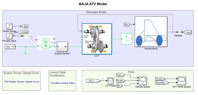
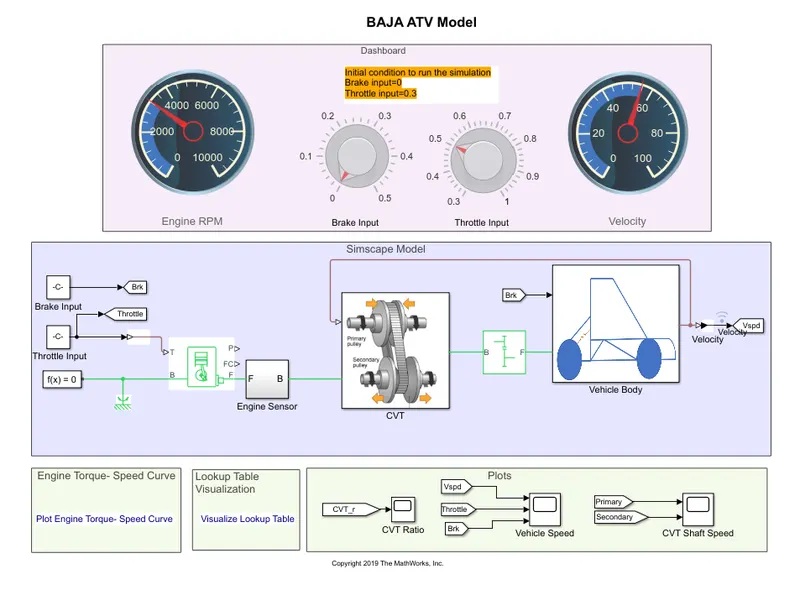
The basic model of the Baja ATV is shown below

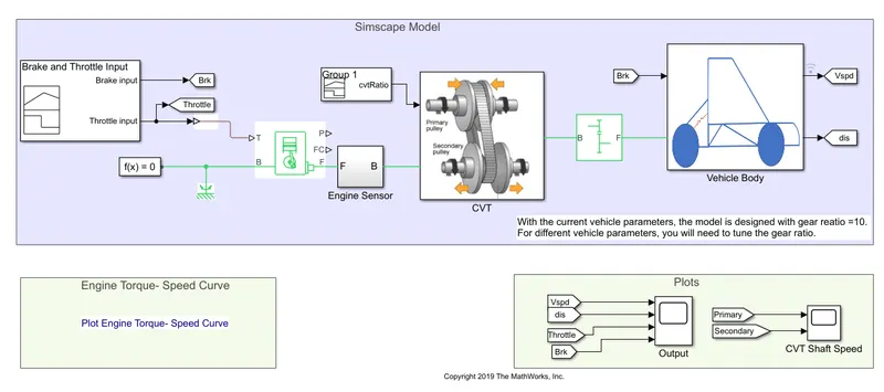
The main components of the given system are:

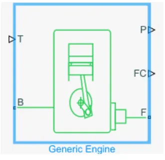
1)GENERIC ENGINE

It represents a system-level model of spark-ignition and diesel engines suitable for use at initial stages of modeling when only the basic parameters are available. The throttle input signal T lies between zero and one and specifies the torque demanded from the engine as a fraction of the maximum possible torque. If the engine speed falls below the Stall speed, the engine torque is blended to zero. If the engine speed exceeds the Maximum speed, the simulation stops and issues an error message.Connections F and B are mechanical rotational conserving ports associated with the engine crankshaft and engine block, respectively. Connections P and FC are physical signal output ports through which engine power and fuel consumption rate are reported.

2) SIMPLE GEAR

Represents a fixed-ratio gear or gear box. No inertia or compliance is modeled in this block. Gear meshing, backlash, and viscous bearing losses can be optionally included.Connections B (base) and F (follower) are mechanical rotational conserving ports. Optionally include thermal effects and expose thermal conserving port H by setting Friction model to a temperature-dependent setting.

3) VEHICLE BODY SUBSYSTEM

The vehicle body sub system consists of the following main blocks

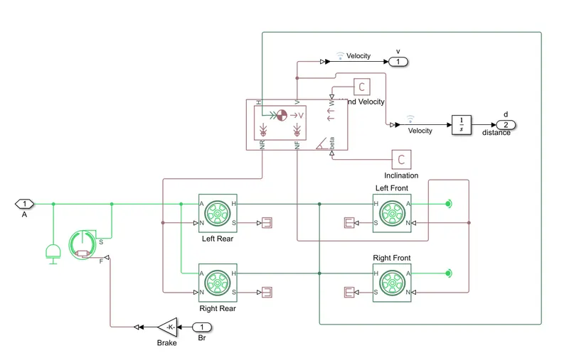
3.1) VEHICLE BODY

Vehiclw body represents a two-axle vehicle body in longitudinal motion. The block accounts for body mass, aerodynamic drag, road incline, and weight distribution between axles due to acceleration and road profile. The vehicle can have the same or a different number of wheels on each axle. Optionally include pitch and suspension dynamics or additional variable mass and inertia. The vehicle does not move vertically relative to the ground.

Connection H is the mechanical translational conserving port associated with the horizontal motion of the vehicle body. The resulting traction motion developed by tires should be connected to this port. Connections V, NF, and NR are physical signal output ports for vehicle velocity and front and rear normal wheel forces, respectively. Wheel forces are considered positive if acting downwards. Connections W and beta are physical signal input ports corresponding to headwind speed and road inclination angle, respectively. If variable mass is modeled, the physical signal input ports CG and M are exposed. CG accepts a two- element vector representing the x and y distance offsets from vehicle CG to additional load mass CG. M represents the additional mass. If both variable mass and pitch dynamics are included, the physical signal port J accepts the inertia of the additional mass about its own CG.

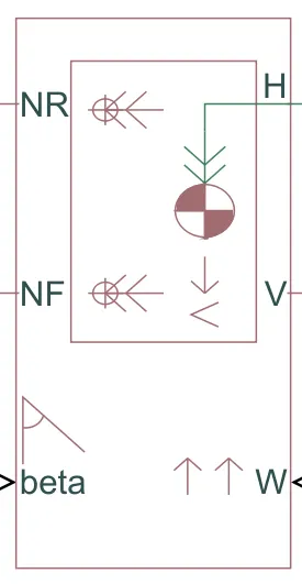
3.2) TIRE

The tyres represents the longitudinal behavior of a highway tire characterized by the tire Magic Formula. The block is built from Tire-Road Interaction (Magic Formula) and Simscape Foundation Library Wheel and Axle blocks.

Connection A is the mechanical rotational conserving port for the wheel axle. Connection H is the mechanical translational conserving port for the wheel hub through which the thrust developed by the tire is applied to the vehicle. Connection N is a physical signal input port that applies the normal force acting on the tire. The force is considered positive if it acts downwards. Connection S is a physical signal output port that reports the tire slip. Optionally expose physical signal port M by setting Parameterize by to Physical signal Magic Formula coefficients. Physical signal port M accepts a four element vector corresponding to the B, C, D, and E Magic Formula coefficients.

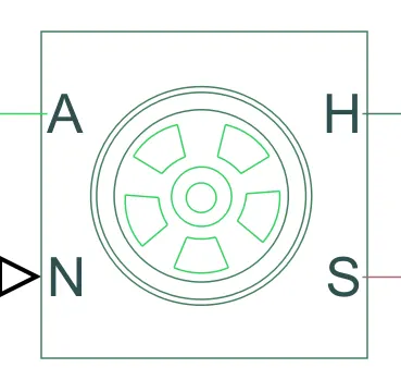
3.3) DOUBLE SHOE BRAKE

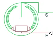
It represents a brake arranged as two pivoted rigid shoes symmetrically installed inside or outside a drum and operated by one actuator. The actuator force causes the shoes to exert a friction torque on a shaft connected to the drum.Connection S is a conserving rotational terminal associated with the drum shaft. Connection F is a physical signal port representing the force input to the actuator. Positive force creates friction torque that resists shaft rotation. Optionally include thermal effects and expose thermal conserving port H by setting Thermal port to Model.

4) CVT SUBSYSTEM

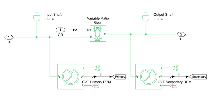
The CVT subsystem consists of :

4.1)INERTIA

The block represents an ideal mechanical rotational inertia.The block has one or two mechanical rotational conserving ports. The difference is purely graphical, as the ports are rigidly linked. The block positive direction is from its port to the reference point. This means that the inertia torque is positive if the inertia is accelerated in the positive direction.

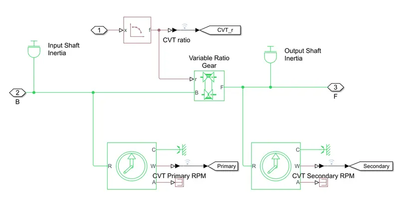
4.2)VARIABLE GEAR RATIO

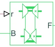
Represents a variable ratio gearbox such as implemented by mechanical belt CVT, electric, or hydraulic transmissions. The physical signal input r defines the ratio of input to output angular shaft velocities.Connections B (base) and F (follower) are mechanical rotational conserving ports. Specify the relation between base and follower rotation directions with the Output shaft rotates parameter.

4.3) IDEAL ROTATIONAL MOTION SENSOR

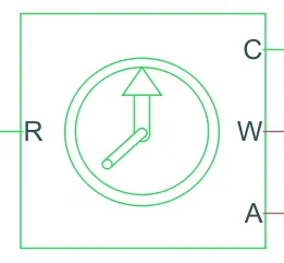
This block measures angular velocity or angle in a mechanical rotational network. The sensor is ideal since it does not account for inertia, friction, delays, energy consumption, and so on.The physical signal ports W and A report the angular velocity and angle, respectively, of port R relative to port C. The measured angular velocity is positive when the angular velocity at port R is greater than the angular velocity at port C.

5) ENGINE SENSOR SUBSYSTEM

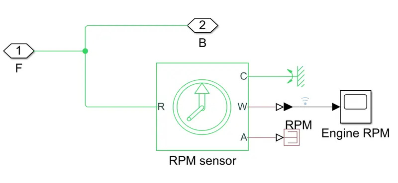
Inorder to track the Generic Engine Crankshaft RPM according to the throttle input, the engine sensor subsystem is used. Hence crankshaft speed is given as input to the engine sensor which analyses the engine RPM with the help of a Rotational Motion Sensor as shown here:

6)SIGNAL BUILDER

The Signal Builder block allows you to create interchangeable groups of piecewise linear signal sources and use them in a model. You can quickly switch the signal groups into and out of a model to facilitate testing. In the Signal Builder window, create signals and define the output waveforms.

1.Baja ATV model without a dashboard

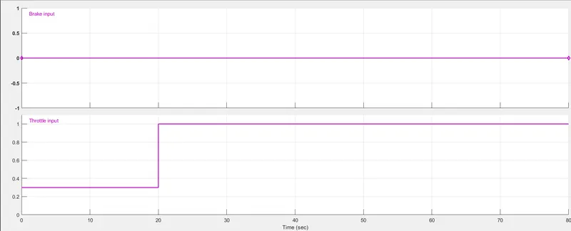
1.1BRAKE AND THROTTLE INPUT

Here brake input is constant throughout the time of 80sec.

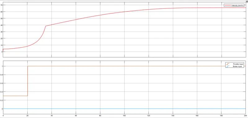
Throttle input is 0.3 for first 20sec, then increased to 1 for the rest of the time.

1.2 CVT GEAR RATIO

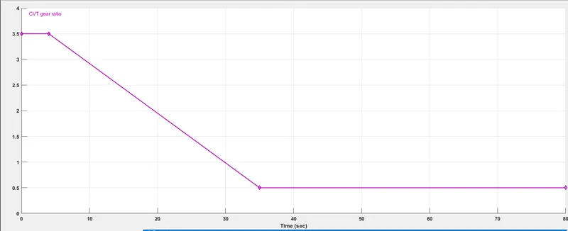
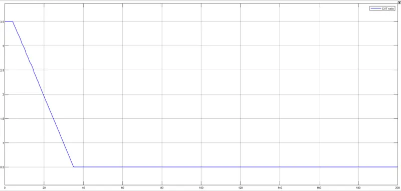
CVT ratio is 3.5 for the first 4sec, then drops down to 0.5 at 35sec and thereafter remains constant for the rest of the time.

OUTPUTS

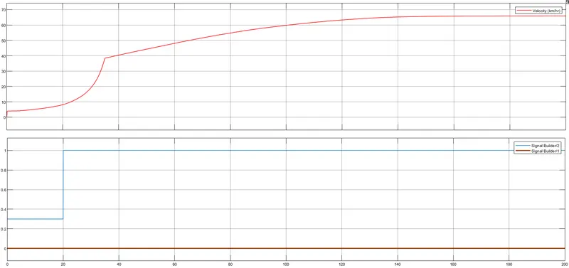
The model was run for 200sec and the corresponding results are obtained

1.3 VELOCITY

Fom the graph, the vehicle attains a maximum speed of 65km/hr at full throttle of 1 and then remains constant. The brakes applied are zero for the entire time range.

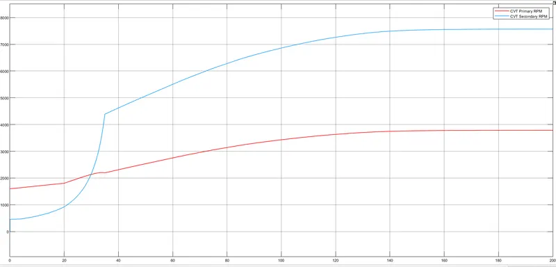
1.4 CVT SHAFT SPEED

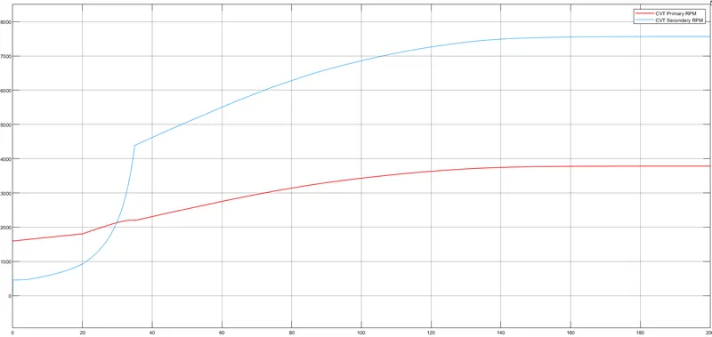
Before 30sec, when CVT ratio is greater than 1, CVT Primary RPM is greater than secondary RPM and after 30sec, when CVT ratio is less than 1, CVT secondary RPM is greater than primary RPM. These values differ with respect to change in gear ratio.

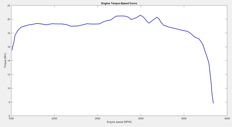
1.5 ENGINE TORQUE SPEED CURVE

1.6 ENGINE SPEED

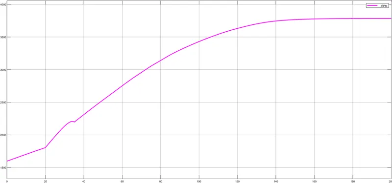
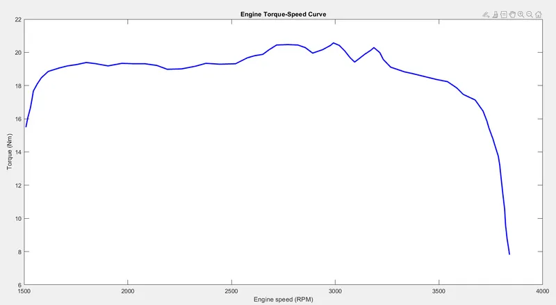
The variation of engine speed (in rpm) with respect to time is shown here. The engine curve settles at an RPM of 3800 , which also matches with the ending point speed in the Torque-speed curve(which is also approximately 3800 rpm)

2.Baja ATV model with a dashboard

In this model, we have a dashboard with knobs to change the brake values and throttle input. The respective meters indicate the RPM nd velocity of the vehicle. The simulation time is set to "inf" so that input parameters could be changed during simulation.

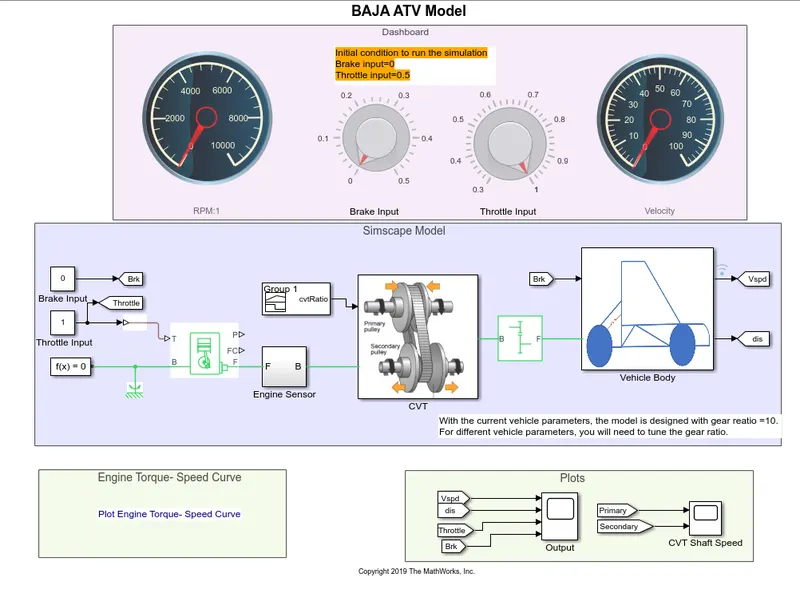
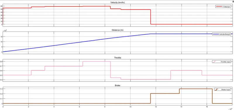
Both brake values and throttle input were changed randomly during simulation to obtain the following results:

2.1 VEHICLE SPEED VARIATIONS AND DISTANCE WITH RESPECT TO THROTTLE AND BRAKE INPUTS

Inputs were given manually to observe the vehicle performance. It is seen that increasing throttle input increases the speed of the vehicle and when brakes are applied 11.5x10^4 sec, there is a decrease in vehicle velocity.

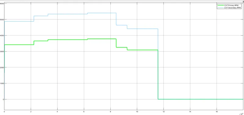
2.2 CVT PRIMARY AND SECONDARY RPM

It can be seen that the CVT primary rpm follows the same pattern as that of secondary rpm. The nature of vehicle velocity and CVT secondary RPM is almost the same as the secondary or driven Pulley is always connected to the vehicle.

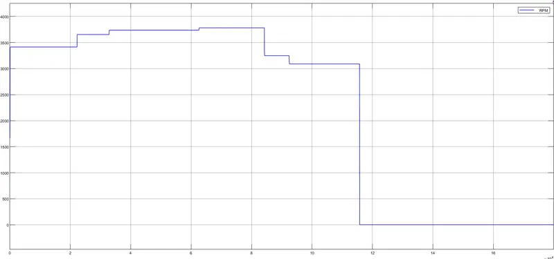
2.3 ENGINE RPM

2.4 ENGINE TORQUE SPEED CURVE

3.Baja ATV model with Look up table and without dashboard

Simulink Model

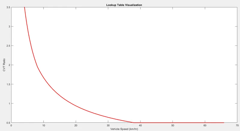
The difference here is that the gear ratio input to the CVT is given using a Look-up table. Also, throttle input and brake are given as step inputs with the same values as in the previous cases. A look up table is an array of data which maps input values to output values. If there is a set of input values, a look-up operation retrieves the corresponding output values from the table. If the look-up table does not define the input values, the block estimates the output values based on nearby table values. The CVT subsystem is shown below in which the look-up table block can be seen.

The look-up table values are as follows:

The CVT ratio graph is obtained as follows:

Vehicle speed variations with Brake and throttle inputs are obtained as shown below:

CVT Primary RPM and CVT Secondary RPM plot:

As the input parameters are the same, the outputs obtained here are similar to first case,(Baja ATV model without a dashboard).

4.Baja ATV model with a look-up table and dashboard

Here, a dashboard with knobs is used to change thr brake and throttle inputs. The look-up table and overall changes in the CVT block are the same as the previous simulink model and hence not repeated again.

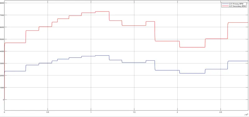
CVT Primary and Secondary RPM

The graph indicates the variations in primary and secondary shaft speed with the changes in throttle and brake inputs during simulation. The initial rise in values are due to the increase in throttle input without the application of brakes. After 1.4, when brakes are applied and throttle input is decreased, the rpm values decreases.

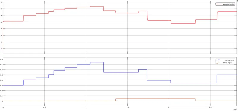
Speed variations with Throttle and brake inputs:

It is clear from the graph that with increase in throttle value, the vehicle speed increases and with an increase in braking value, the vehicle velocity decreases. The inputs were changed randomly during simulation using the knobs and the following vehicle performance was observed.

CONCLUSION

We have successfully analysed the given model of BAJA ATV using matlab and observed the various outputs obtained in different modes. Thus we could also incorporate real component data (engine, vehicle dynamics,CVT etc) into the models, and can use sufficient realistic data to model real-world conditions.

REFERENCES

1. https://in.mathworks.com/matlabcentral/fileexchange/70576-baja-all-terrain-vehicle-atv-model

2.https://en.wikipedia.org/wiki/All-terrain_vehicle

3.https://en.wikipedia.org/wiki/Baja_SAE

4.https://www.youtube.com/watch?v=gOFweQcz0XI

5.https://in.mathworks.com/help/physmod/sdl/ref/vehiclebody.html