Project

 Carry out a system-level simulation of an all-terrain vehicle and prepare a technical report explaining the model properties & comments on the results.

Aim:

To carry out a system-level simulation of an all-terrain vehicle and prepare a technical report explaining the model properties & comments on the results.

Theory:

• System-level simulation: System-level simulation (SLS) is a collection of practical methods used in the field of systems engineering, in order to simulate, with a computer, the global behaviour of large cyber-physical systems.
  
  
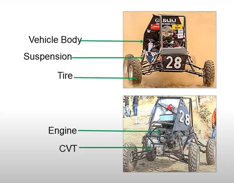
• All-Terrain Vehicles: An all-terrain vehicle(ATV), also known as a light utility vehicle (LUV) is a vehicle that travels on low-pressure tires, with a seat that is straddled by the operator, along with handlebars for steering control. As the name implies, it is designed to handle a wider variety of terrain than most other vehicles.
  
  
  
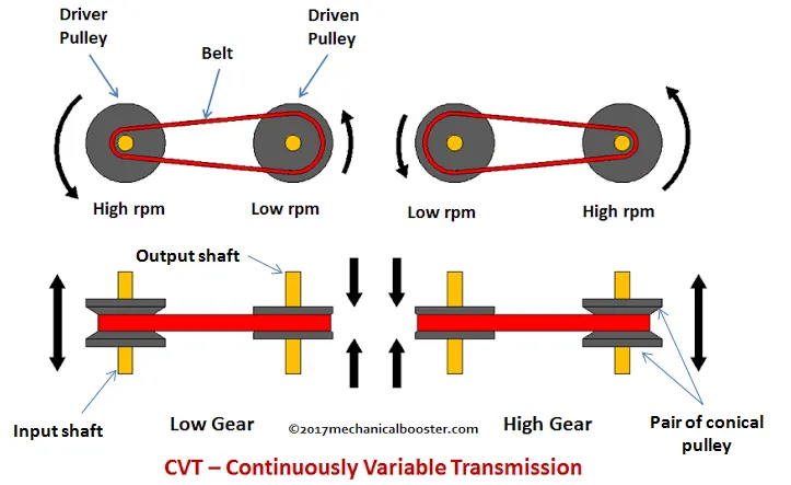
• Continuously Variable Transmission: A continuously variable transmission (CVT) is an automatic transmission that can change seamlessly through a continuous range of gear ratios. This contrasts with other transmissions that provide a limited number of gear ratios in fixed steps. The flexibility of a CVT with suitable control may allow the engine to operate at a constant RPM while the vehicle moves at varying speeds.
  
  
  
  
  

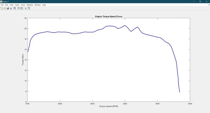
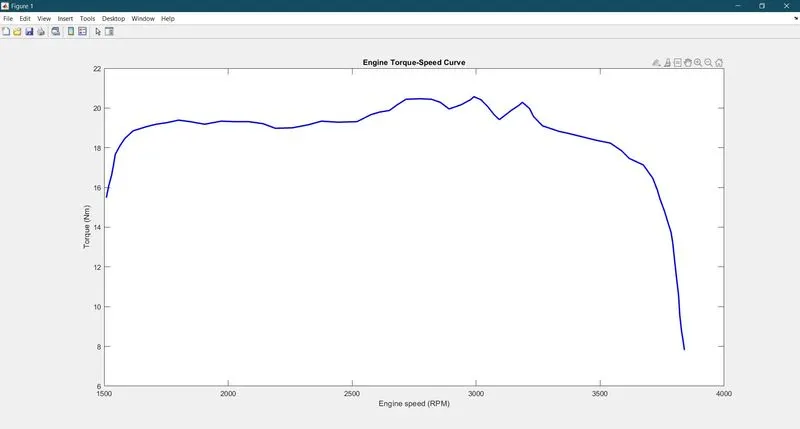
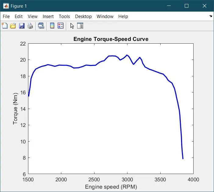
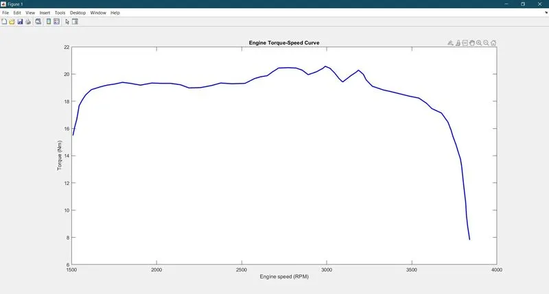
This submission contains a set of models created with Simulink, Simscape, and Simscape Driveline. More specifically, the file contained includes BAJA ATV model with Continuously Variable Transmission (CVT). These models show how to build an ATV with CVT which is mostly used in BAJA competitions. Simscape and Simscape Driveline have been used to complete the system. The engine data used in the model is provided as an image which shows the Engine Speed (RPM) Vs Torque curve.

Simscape model for BAJA ATV:

 CASE 1: ATV with No DASHBOARD:-

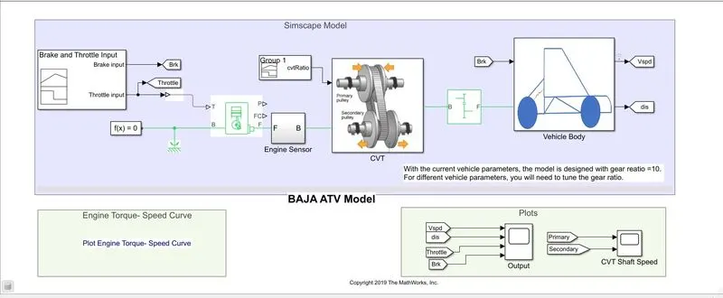
Components:

1. Brake & Throttle input and CVT ratio:
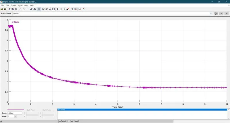
   This block is build using a signal builder where the throttle & brake inputs and CVT ratio are provided. The Signal Builder block allows you to create interchangeable groups of piecewise linear signal sources and use them in a model. You can quickly switch the signal groups into and out of a model to facilitate testing. In the Signal Builder window, create signals and define the output waveforms.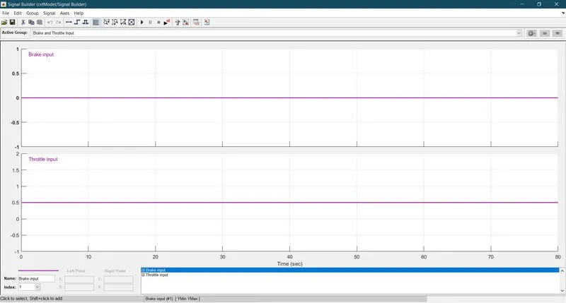
   
2. Generic Engine block:
   Represents a system-level model of spark-ignition and diesel engines suitable for use at initial stages of modelling when only the basic parameters are available. Optional idle speed and red line controllers are included.
   
   
3. Engine sensor:
   It is a subsystem which is used to measure the RPM of shaft. It is achieved using an Ideal Rotational motion sensor block. This block measures angular velocity or angle in a mechanical rotational network. The sensor is ideal since it does not account for inertia, friction, delays, energy consumption, and so on.
   
   
4. Simple Gear:
   Represents a fixed-ratio gear or gear box. No inertia or compliance is modelled in this block. You can optionally include gear meshing and viscous bearing losses.
   
   
5. Solver configuration:
   Defines solver settings to use for simulation.
   
   
6. CVT Subsystem:

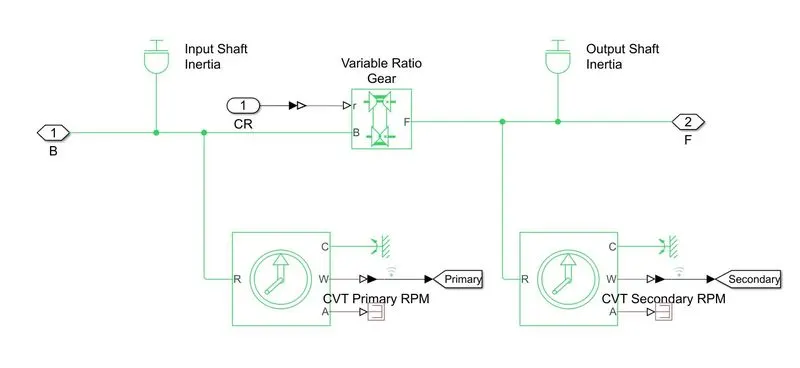
• Variable-Ratio Transmission:
  Represents a variable ratio gearbox such as implemented by mechanical belt CVT, electric, or hydraulic transmissions. The physical signal input r defines the ratio of input to output angular shaft velocities.
  
  
• Inertia:
  The block represents an ideal mechanical rotational inertia.
• Ideal Rotational Motion Sensor:
  This block measures angular velocity or angle in a mechanical rotational network. The sensor is ideal since it does not account for inertia, friction, delays, energy consumption, and so on.
  
  
• Mechanical Rotational Reference:
  This block represents a mechanical rotational reference point, that is, a frame or a ground. Use it to connect mechanical rotational ports that are rigidly affixed to the frame (ground).

 7. Goto Block:
Send signals to From blocks that have the specified tag. If tag visibility is 'scoped', then a Goto Tag Visibility block must be used to define the visibility of the tag. The block icon displays the selected tag name (local tags are enclosed in brackets, [], and scoped tag names are enclosed in braces, {}).

8. From Block:
Receive signals from the Goto block with the specified tag. If the tag is defined as 'scoped' in the Goto block, then a Goto Tag Visibility block must be used to define the visibility of the tag. After 'Update Diagram', the block icon displays the selected tag name (local tags are enclosed in brackets, [], and scoped tag names are enclosed in braces, {}).

9. Vehicle Body Subsystem: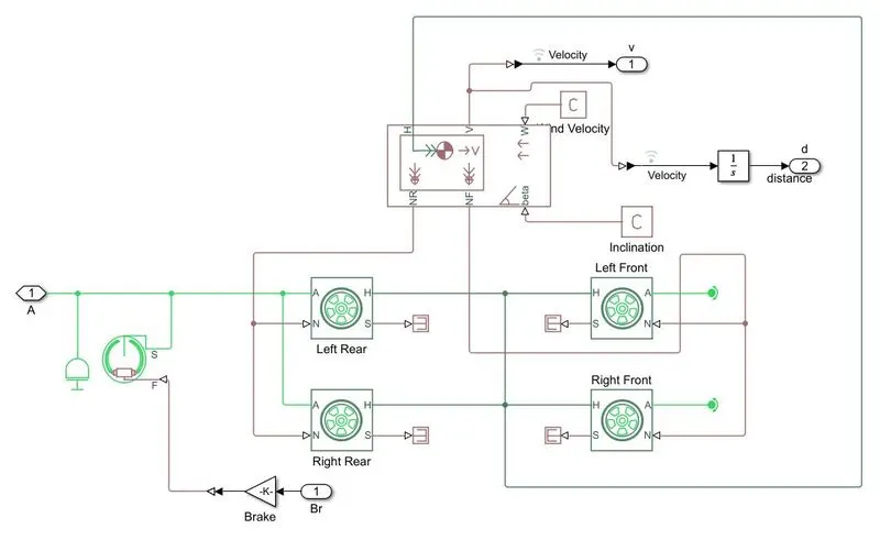

• Vehicle Body Block:
  Represents a two-axle vehicle body in longitudinal motion. The block accounts for body mass, aerodynamic drag, road incline, and weight distribution between axles due to acceleration and road profile. The vehicle can have the same or a different number of wheels on each axle. Optionally include pitch and suspension dynamics or additional variable mass and inertia. The vehicle does not move vertically relative to the ground.
  
  
• Tire:
  Represents the longitudinal behaviour of a highway tire characterized by the tire Magic Formula. The block is built from Tire-Road Interaction (Magic Formula) and Simscape Foundation Library Wheel and Axle blocks. Optionally, the effects of tire inertia, stiffness, and damping can be included.
  
  
• Double-shoe brake:
  Represents a brake arranged as two pivoted rigid shoes symmetrically installed inside or outside a drum and operated by one actuator. The actuator force causes the shoes to exert a friction torque on a shaft connected to the drum.
  
  
• PS Terminator:
  Use this block to terminate physical signal outputs. Unconnected physical signal output ports do not generate warnings, but connection to a PS Terminator can be used to indicate that the signal was not inadvertently left unconnected.
  
  
• PS Constant:
  This block creates a physical signal constant.
  
  
• Inertia:
  The block represents an ideal mechanical rotational inertia.

Working:

1. In the case 1, the simulation is set for Stop time =200
2. In the case 1, model is analysed using a Signal builder block. i.e., the signal builder is used to provide to provide the input signals which are, Throttle, Brake and CVT ratio.
   
   
3. The signals are fed to the Generic Engine, which is the simplest form of engine system and connected via Solver configuration block.
   
   
4. The output signals are sent to the Engine sensor or RPM sensor to analyse the speed of engine shaft.
   
   
5. The measured signal is given to one input of the CVT subsystem and other input is given by the previously mentioned Signal builder’s CVT ratio
   
   
6. Then, the output of CVT is connected to a Simple gear for required gear ratio. With the current vehicle parameters, the model is designed with gear ratio =10.
   
   
7. Finally, the output with desired gear ratio is fed to the Vehicle body subsystem.
   
   
8. The analysis is made through Goto and From blocks through a scope.

CASE 2: ATV with DASHBOARD

Components:

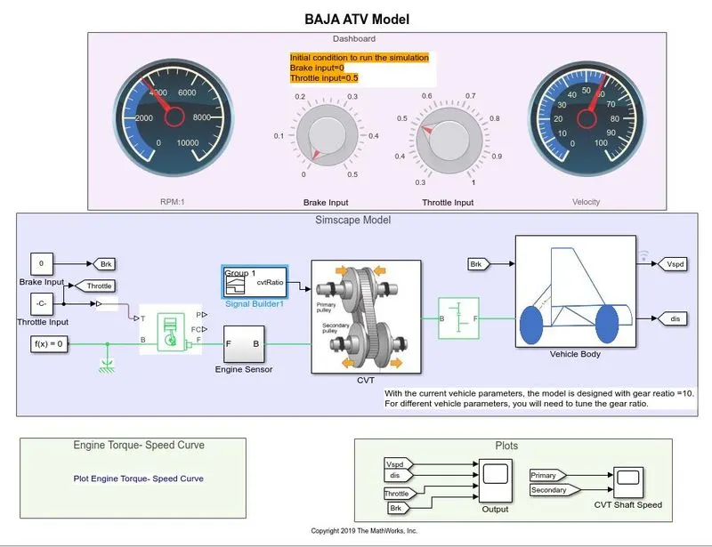
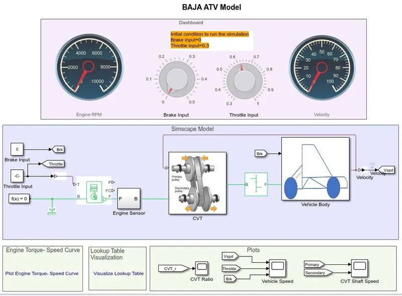
Majority of the components are like that of Case 1. The only change in here is that we use Dashboard controllers for throttle and brakes to change the Input manually rather than pre-set value from signal builders.

1. Knob:
   Set a value to tune parameters or variables.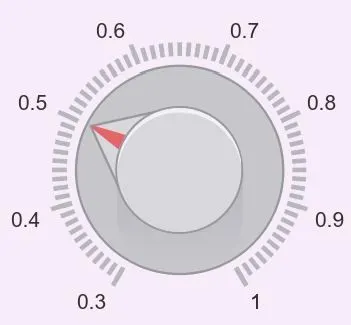
   

Circular Gauge:
Display an input value on a customized gauge.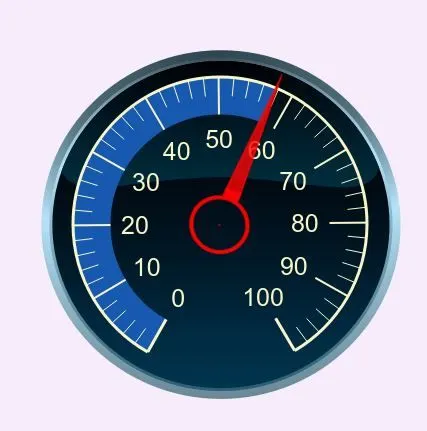

Working:

1. The working is also like Case 1 except for the dashboard controls.
   
   
2. Also, the simulation is set to inf
   
   
3. Here, the Initial condition to run the simulation is set as Brake input=0 and Throttle input=0.5
   
   
4. Once, the simulation is started, the values of brake and throttle are manually controlled to find the readings.
   

CASE 3: ATV with No DASHBOARD using Lookup Table

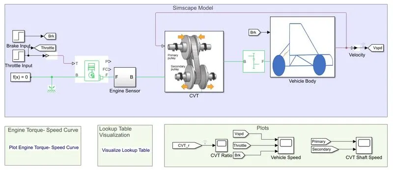
Components:

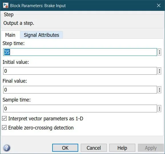
• The inputs are step signals instead of deigning on Signal Builder.
  
  
  • Throttle input-
    
    
    
    
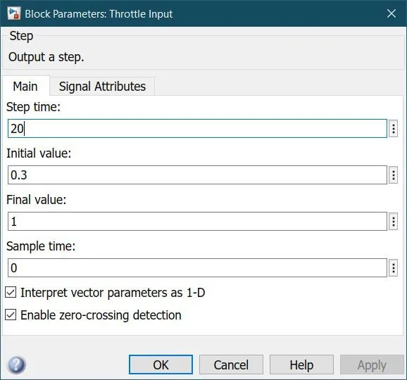
  • Brake input-
    
    
    
    
• 1-D Lookup Table:
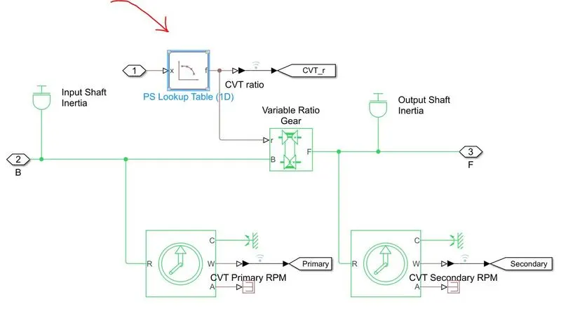
  This block represents a physical signal converter whose input-output relationship is specified by a lookup table. The table grid must be in strictly ascending or strictly descending order, but the spacing can be non-uniform.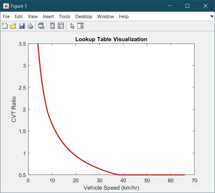
  
  
  

Working:

1. The Step input signals provide the Throttle and Brake values.
   
   
2. Also, the simulation is set to stop time = 200
   
   
3. Here, the lookup table works as a Feedback loop for the CVT system by arranging the gear ratio needed for the CVT.
   
   
4. Here, due to the introduction of 1-D lookup table, the system works as closed loop.
   
   
5. Thus, the gear ratio changes of CVT according to the input values and the tyre requirement.
   
   

CASE 4: ATV with DASHBOARD using Lookup Table

Components:

Majority of the components are like that of Case 2. The only change in here is that we use Dashboard controllers for throttle and brakes to change the Input along with 1-D look up table for a feedback loop.

• 1-D Lookup Table:
  This block represents a physical signal converter whose input-output relationship is specified by a lookup table. The table grid must be in strictly ascending or strictly descending order, but the spacing can be non-uniform.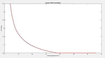
  
  
  
  

Working:

1. The operation is almost like the Case 2 while controlling the dashboard.
   
   
2. Also, the simulation is set to stop time = inf
   
   
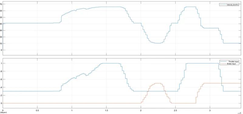
3. The Throttle knob can be varied from 0.3 to 1.0 while the Brake knob can be varied from 0.0 to 0.5
   
   
4. The initial condition for knobs to be set as Throttle = 0.3 and Brake = 0.0
   
   
5. Here, due to the introduction of 1-D lookup table, the system works as a completely closed loop.
   
   
6. Thus, the gear ratio changes of CVT according to the input values and the tyre requirement.
   
   

Observations:

• Case 1:

              1. Engine Torque- Speed Curve-

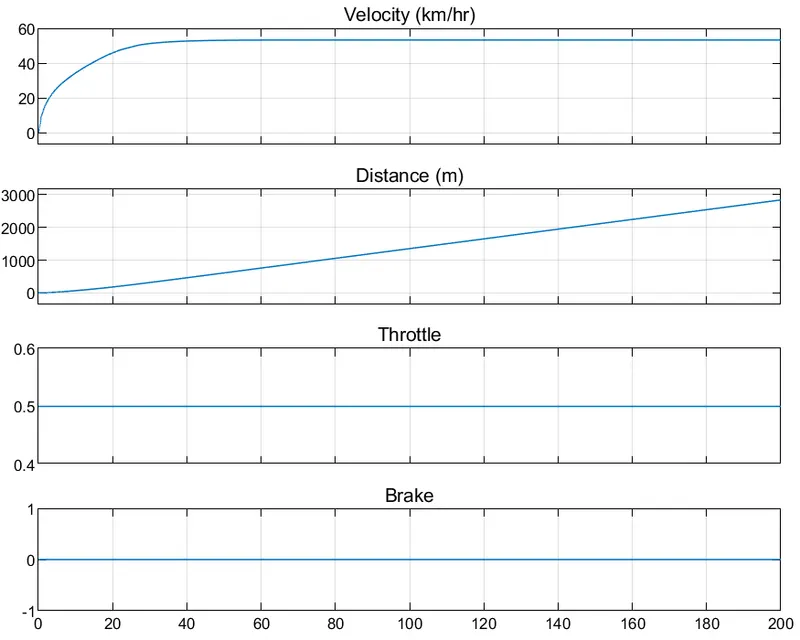
              2. Output Chara for Velocity, Distance, Speed and Brake

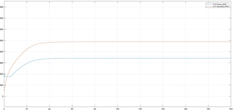
              3. CVT Shaft Speed-

• Case 2:

              1. Engine Torque- Speed Curve-

             2. Output Chara for Velocity, Distance, Speed and Brake

              3. CVT Shaft Speed-

• Case 3:

              1. Engine Torque- Speed Curve-

 2. Output Chara for Velocity, Distance, Speed and Brake

3. CVT Shaft Speed

• Case 4
  
  

1. Engine Torque- Speed Curve-
   
   
   
2. CVT Ratio-
   
   
   
   
3. Output Chara for Velocity, Distance, Speed and Brake-
   
   
   
4. CVT Shaft Speed-
   
   

1. Engine Torque- Speed Curve-
   
   All the 4 cases are provided with the exact Engine Torque – Speed Chara
   
   
   
2. Output Chara for Velocity, Speed and Brake-
   
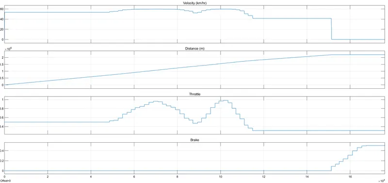
      -In Case 1, For the given Throttle = 0.5 and Brake input = 0, the velocity exponentially rise from 0 to almost 60 in 20 sec and remains constant for remaining time.
   
      -In Case 2, the initial position of knob of throttle is at 1 and brake at 0, that is the vehicle is on move. when the knob value of throttle is increased furthur, there is a slight increment on the velocity and respond to the knob accordingly. When the Throttle knob is turned to zero, the velocity decreases and when the brake input knob is increased, the velocity falls to zero.
   
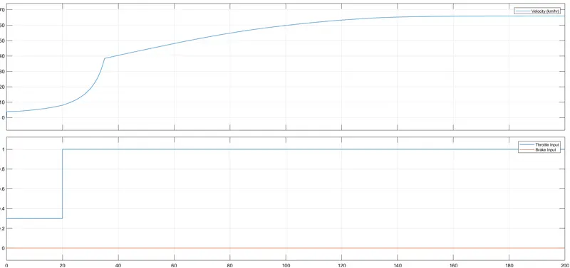
      -In Case 3, the throttle input is kept at 0.3 until 20 secs and increased to 1.0 for the rest of the simulation time whilekeeping the brake input at zero for the entire duration. Here the velocity increases exponentinally for almost 40 secs and later at a gradual and smooth pace
   
      -In Case 4, it is evident from the graph that, the velocity responds with some latency but smoothly. the response is not that spontaneous due to the presence of look up table, rather a smooth comfortable response. Here the initial conditions for throttle input is = 0.3 and for brake is = 0. and for this input, the velocity is almost constant at 40. When though, after  Throttle knob value is increased vigoursly, the velocity seems less affected and velocity seems to increase gradually. Even for the braking, the velocity seems to respond smoothly.
   
   
   
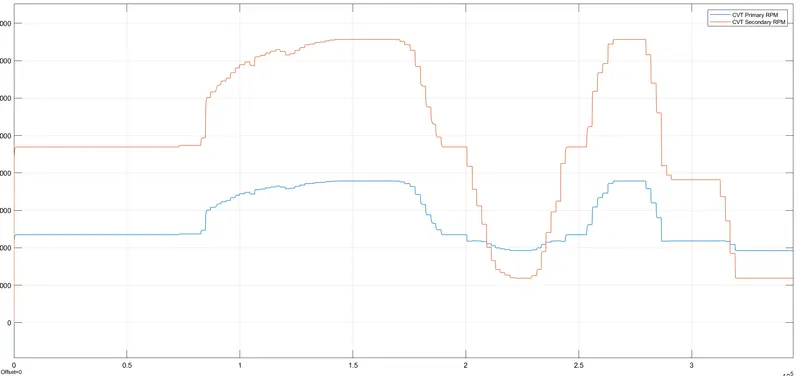
3. CVT Shaft Speed-
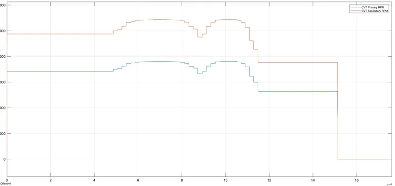
      -In Case 1, primary shaft rpm is higher than secondary shaft rpm at starting due to high torque demand. but after 5 sec, secondary rpm crosses the primary rpm because primary rpm shaft has higher radius than secondary rpm shaft
   
      -In Case 2, the secondary CVT shafts rotates at higher rpm compared to primary shaft RPM, and increases the RPM values proportionally to the throttle input and brake input knob. Both the RPM falls to zero when brake is applied. 
   
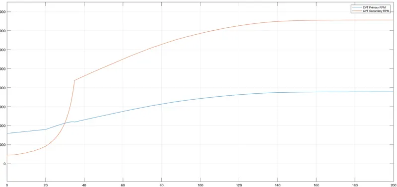
      -In Case 3, the secondary CVT shaft rpm behaves similar to the velocity for almost all the time. but at the starting, thr primary rpm value is higher than that of the secondary and after 30 secs the rpms crosses.
   
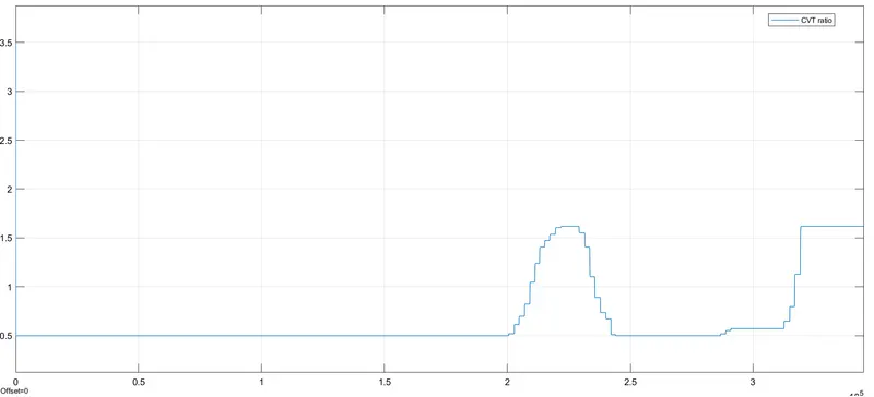
      -In Case 4, the primary and secondary shaft rpm are proportional for the provided input throttle. Even when the throttle is increased, the gear ratio seems to increase in discrete values
   

Conclusion:

• Successfully studied and carried out the system-level simulation of an all-terrain vehicle
  
  
• Analysed the effect the Throttling and Braking on CVT and output Velocity
  
  
• Analysed the relationship between the primary and secondary CVT shaft speeds and its effect on velocity
  
  
• Analysed the difference between Open-loop and Closed-loop CVT system.
  
  
• Understood the importance of Lookup table in CVT system.

Reference:

1. https://www.mathworks.com/matlabcentral/fileexchange/70576-baja-all-terrain-vehicle-atv-model
2. https://en.wikipedia.org/wiki/Continuously_variable_transmission
3. https://en.wikipedia.org/wiki/System-level_simulation
4. https://en.wikipedia.org/wiki/Baja_SAE
5. https://www.youtube.com/watch?v=gOFweQcz0XI