Project

AIM:

To study the BAJA ATV simulation and prepare a detailed technical report on various model’s properties.

OBJECTIVES:

• Carry out a system level simulation of an All-Terrain vehicle for 4 model properties and comment on the results.
• Observe the results for given CVT data for open loop and closed loop layout systems.

THEORY:

All-Terrain Vehicle

ATV means an All-Terrain Vehicle which is specially designed for an off-road driving with very rough terrain, jumps, manoeuvrability and endurance. The design process of this single-person vehicle is iterative and based on several engineering and reverse engineering processes. The designing work is initiated to achieve the best standardized as well as optimized design possible. Specifications lay down by the standard specifications available foremost concern while designing and selection of the parts.

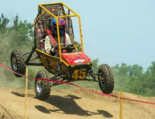
Main Components of BAJA ATV

• Engine
• continuously variable transmission (CVT)
• Suspension
• Tires
• Vehicle Body

Continuously Variable Transmission

A continuously variable transmission (CVT) is an automatic transmission that can change seamlessly through a continuous range of gear ratios. This contrasts with other transmissions that provide a limited number of gear ratios in fixed steps. The flexibility of a CVT with suitable control may allow the engine to operate at a constant RPM while the vehicle moves at varying speeds. CVTs are used in automobiles, tractors, motor scooters, snow mobiles and earthmoving equipment’s.

The most common type of CVT uses two pulleys connected by a belt or chain; however, several other designs have also been used at times.

Working principal of CVT system

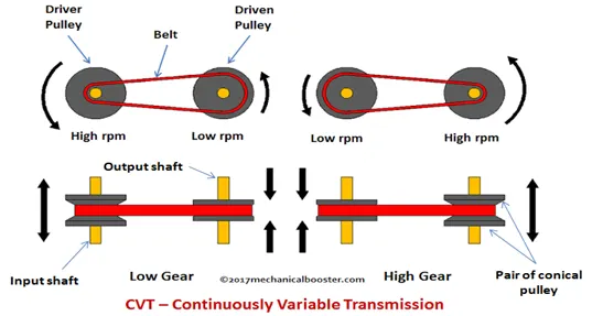
Most CVT systems works through a pully system, consists of cones at each pully connected via a chain belt. The cones can move increase or decrease the belt diameter to change gear ratios, allow for quick shifting into the needed ratio for increased power and boost fuel economy.

Where one pully in the CVT is connected to the engine and the other directs power to the wheels. The width of the pulleys change based on the needed power, as one gets larger, the other gets smaller. This allows the CVT to deliver strong and seamless acceleration.

4 Case studies

Case study-1: Open loop, Baja AVT model.

Case study-2: Open loop, Baja AVT model with Dashboard.

Case study-3: Closed loop, Baja AVT mapped model (Using Look Up Table).

Case study-4: Closed loop, Baja AVT mapped model with Dashboard (Using Look Up Table).

Case study-1: Open loop, Baja AVT model:

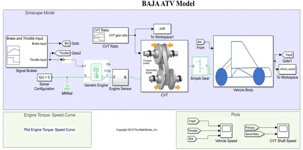
Main Simulink blocks used to build the model

Signal Builder:

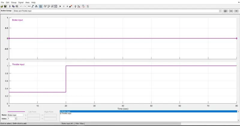
Here, Brake and Throttle input values are given in the form of plot as shown below and this block is connected to Generic engine block.

Were

• Brake input value is ‘0’
• Throttle input value at initial condition is ‘0.3’ for 20 seconds and the value is ‘1’ after the 20 seconds.

Generic Engine:

Represents a system-level model of spark-ignition and diesel engines suitable for use at initial stages of modelling when only the basic parameters are available. Optional idle speed and red line controllers are included.

The throttle input signal T lies between zero and one and specifies the torque demanded from the engine as a fraction of the maximum possible torque. If the engine speed falls below the Stall speed, the engine torque is blended to zero. If the engine speed exceeds the Maximum speed, the simulation stops and issues an error message.

Connections F and B are mechanical rotational conserving ports associated with the engine crankshaft and engine block, respectively. Connections P and FC are physical signal output ports through which engine power and fuel consumption rate are reported.

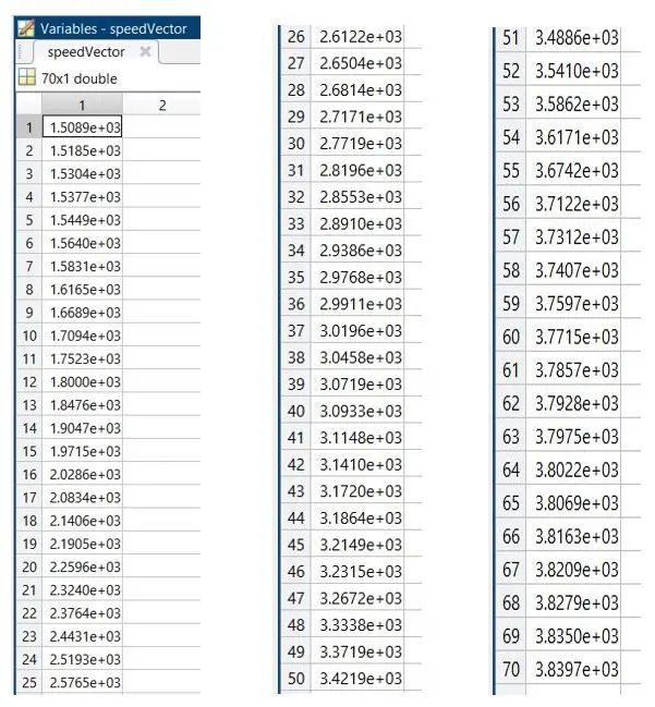
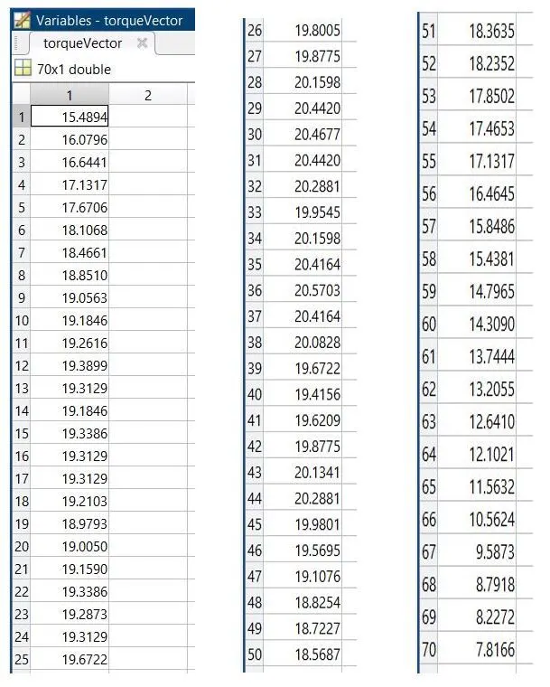
The values of speedVector and torqueVector are assigned in the MATLAB program in the form of array data set.

Engine Sensor:

Engine Sensor is connected with Generic Engine. Engine Sensor contains Ideal Mechanical Rotational Sensor that converts an across variable measured between two mechanical rotational nodes into a control signal proportional to angular velocity or angle. Connections R and C are mechanical rotational conserving ports and connections W and A are physical signal output ports for velocity and angular displacement, respectively.

Simple Gear:

Engine is Connecting to CVT with Simple Gear ratio for Speed Reduction.

Continuously Variable Transmission:

The main components of Continuously Variable Transmission (CVT) are:

• Belt
• Variator
• Primary Pulley
• Secondary Pulley

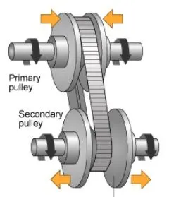
If Variator of Primary Pulley goes outward and Secondary pulley goes inward it will lead to Speed Reduction.

Rp < Rs

If Variator of Primary Pulley goes inward and Secondary Pulley goes Outward it will lead to Overdrive.

Rp > Rs

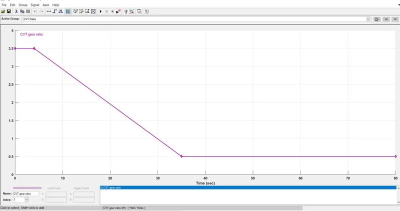
CVT Ratio:

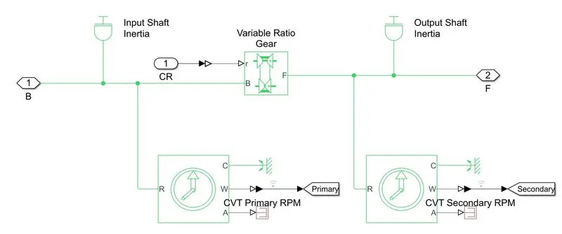
The CVT Ratio Block is connected with CVT by giving random ratio values to get the value of velocity for those random CVT ratio.

Vehicle Body:

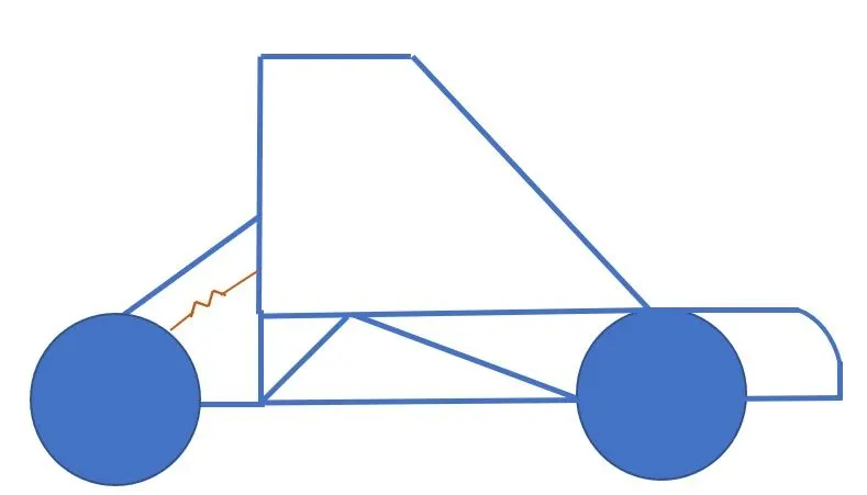
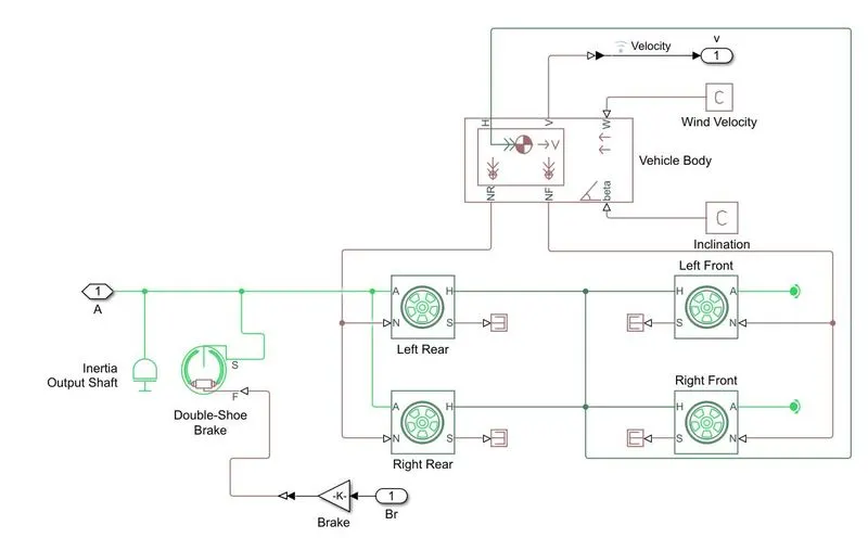
Vehicle Body represents a two-axle vehicle body in longitudinal motion. The block accounts for body mass, aerodynamic drag, road incline, and weight distribution between axles due to acceleration and road profile. The vehicle can have the same or a different number of wheels on each axle. Optionally include pitch and suspension dynamics or additional variable mass and inertia. The vehicle does not move vertically relative to the ground. Vehicle Body contains Two Front wheel and Two Rear Wheel which is connected with Inertia Output Shaft and Double Shoe Brake.

RESULTS:

Plot Engine Torque - Speed Curve:

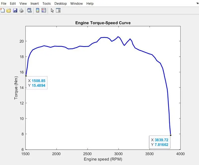
From the above plot we can observe that Maximum Velocity reaches at 3839.72 RPM when the Torque is 7.81662 Nm. So, the Vehicle Speed will depend on CVT Ratio.

Vehicle Speed Plot:

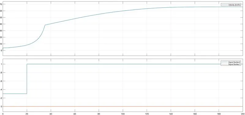
From the above Plot, Brake input is 0 and Throttle input is 0.3 for 20 seconds Velocity will reach 20 and by increasing the Throttle input value to 1 and keep it constant, then velocity value will increase and it reaches the maximum velocity.

CVT Shaft Speed Plot:

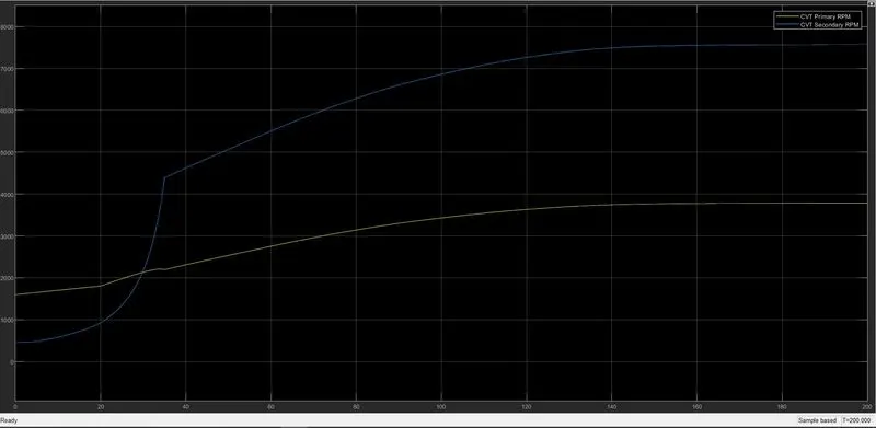
In Continuously Variable Transmission (CVT) if Variator of Primary Pulley goes outward and Secondary pulley goes inward it will lead to Speed Reduction. Primary Pulley radius decreases and Secondary Pulley radius increases. So, Speed of Secondary Pulley is greater than primary Pulley.

Rp < Rs

Engine Speed Plot:

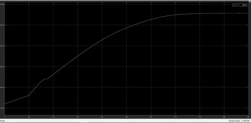
From the above Plot, when the Brake input is 0 and Throttle input is 0.3 for 20 seconds, Engine Speed will decrease at the beginning because of increasing gear ratio which increases the torque and by increasing the Throttle input value to 1, then Engine Speed value will increase and it reaches the maximum Speed.

Case study-2: Open loop, Baja AVT model with Dashboard:

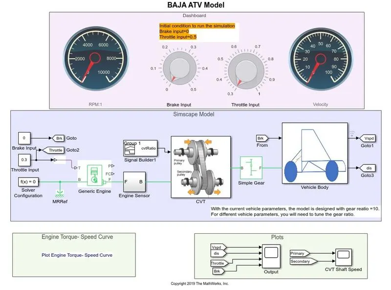
In this model dashboard is added to connect RPM-Speed gauge, Brake input gauge, Throttle input gauge and Velocity gauge. Where the Brake input is 0, Throttle input is 0.3 for Initial Conditions.

Dashboard is connected with BAJA All terrain Vehicle using CVT in Simulink Model. With the help of Dashboard, variation of Speed and Velocity will display in the RPM:1 gauge and Velocity gauge, while running the Simulation, when the input is given through brake and throttle gauges.

RPM gauge refers the Speed of the Primary & Secondary Pulley and Velocity gauge refers the Speed of the Vehicle.

CVT Ratio Plot:

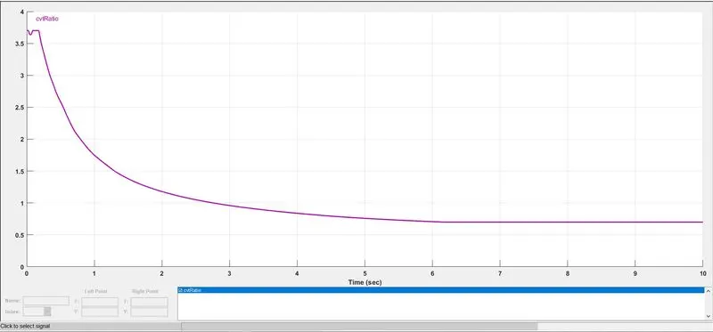
RESULTS:

Given inputs through the brake and throttle input gauges.

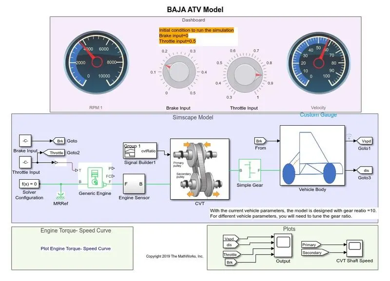
By setting running time value as "inf" and Run the Simulation. While simulation is running, throttle input value & Brake Input Value can change in Throttle input gauge & Brake Input gauge in the dashboard and will analyse the variation of RPM and velocity in the RPM gauge and Velocity Gauge.

Vehicle Speed Plot:

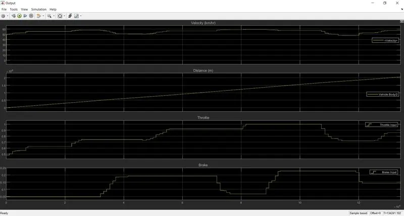
From the above Vehicle Speed plot, we can observe that by increasing the throttle input value, it will increase the Velocity and vice-versa and by increasing the brake input value it will decrease the Velocity and vice-versa. When the throttle input value remains constant then velocity will be constant.

CVT Shaft Speed Plot:

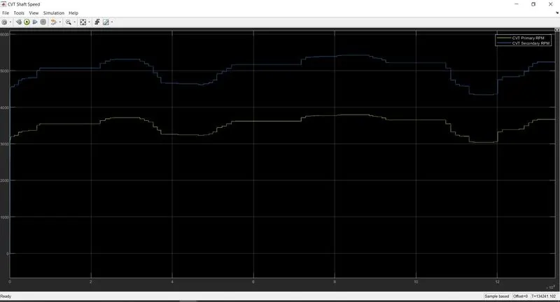
From the above CVT Shaft Speed plot, we can observe that by increasing the throttle input value, it will increase the RPM of the Primary & Secondary Pulley and by increasing the brake input value it will decrease the RPM of the Primary & Secondary Pulley.

Engine Speed Plot:

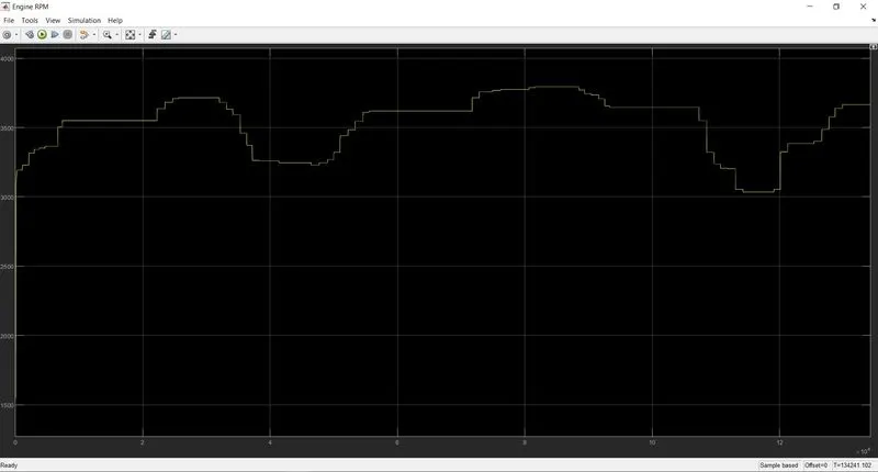
From the above Engine Speed plot, we can observe that by increasing the throttle input value, it will increase the Engine Speed and by increasing the brake input value it will decrease the Engine Speed.

Case study-3: Closed loop, Baja AVT mapped model (Using Look Up Table):

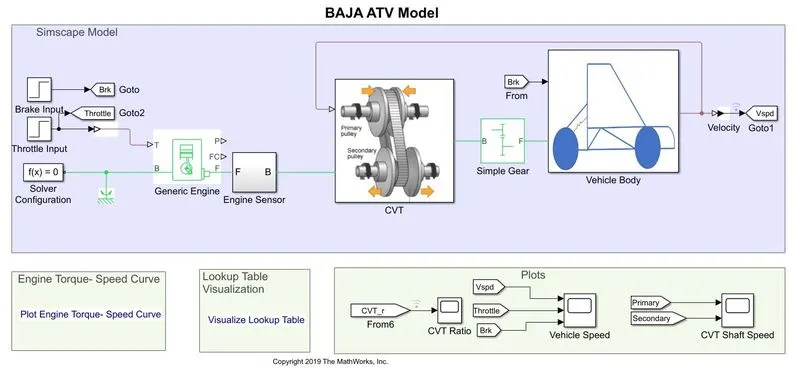
From the above model Look Up table data has been assigned as input to the CVT instead of giving CVT ratio data set. For Giving input of Look up table by creating a program in the MATLAB and Data has been assigned as input to the CVT.

MATLAB Program for Look Up Table

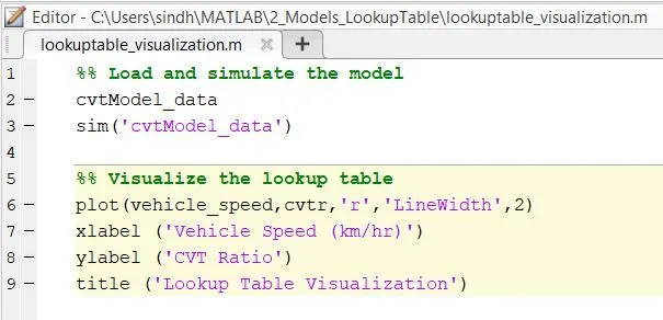
First run this program in MATLAB, the output plot will be the look up table.

Workspace

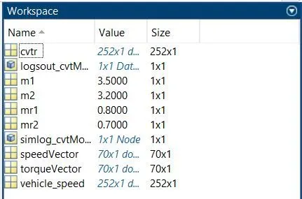
Look Up Table data has assigned as cvtr in the workspace

Look Up Table Plot:

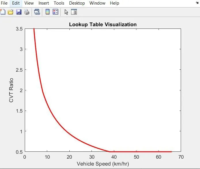
After creating Look Up Table data, give the data as input to the CVT

RESULTS:

CVT Ratio Plot (Look Up Table Data):

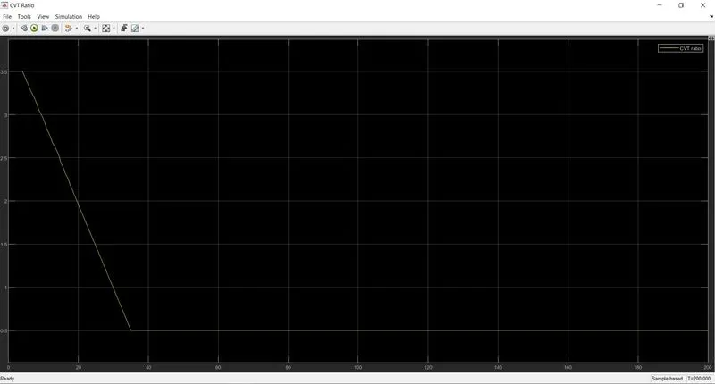
The above plot shows the value of Look Up Table input data given to the CVT.

Vehicle Speed Plot:

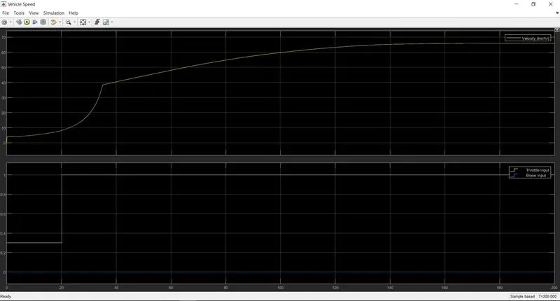
From the above Plot, Brake input is 0 and Throttle input is 0.3 for 20 seconds. Velocity will reach 20 and by increasing the Throttle input value to 1, then velocity value will increase and it reaches the maximum velocity.

CVT Shaft Speed Plot:

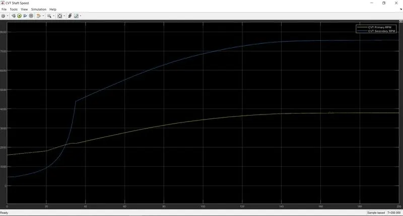
In Continuously Variable Transmission (CVT) if Variator of Primary Pulley goes outward and Secondary pulley goes inward it will lead to Speed Reduction. Primary Pulley radius decreases and Secondary Pulley radius increases. So, Speed of Secondary Pulley is greater than primary Pulley.

Rp < Rs

Engine Speed Plot:

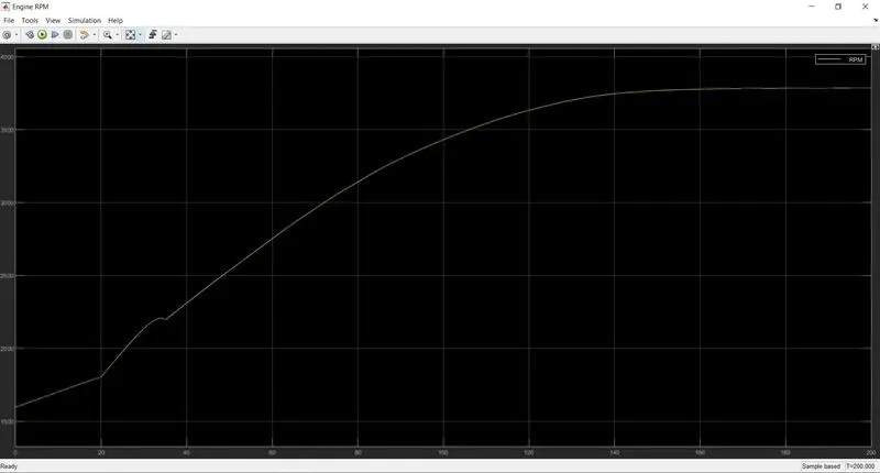
From the above Plot, Brake input is 0 and Throttle input is 0.3 for 20 seconds, Engine Speed will decrease at the beginning because of increasing gear ratio which increases the torque and by increasing the Throttle input value to 1, then Engine Speed value will increase and it reaches the maximum Speed.

Case study-4: Closed loop, Baja AVT mapped model with Dashboard (Using Look Up Table):

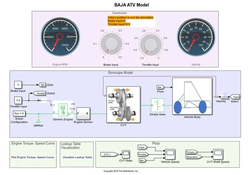
In this model dashboard is added to connect RPM-Speed gauge, Brake input gauge, Throttle input gauge and Velocity gauge. Where the Brake input is 0, Throttle input is 0.3 for Initial Conditions.

For the above model Look Up table data has been assigned as input to the CVT instead of giving CVT ratio data set. Loop up table is plotted, by creating a program in the MATLAB and Data has been assigned as input to the CVT.

RESULTS:

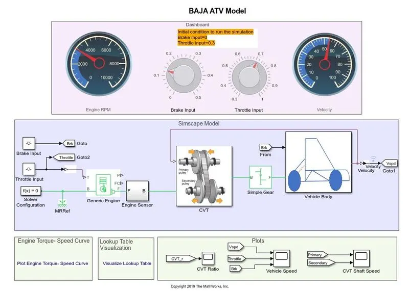
By setting running time value as "inf" and Run the Simulation. While simulation is running, throttle input value & Brake Input Value can change in Throttle input gauge & Brake Input gauge in the dashboard and will analyse the variation of RPM and velocity in the RPM gauge and Velocity Gauge.

CVT Ratio Plot (Look Up Table Data):

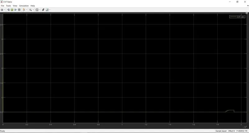
From the above plot, CVT Ratio will vary by changing the Throttle input gauge. If Throttle value increases CVT ratio decreases and vice-versa.

Vehicle Speed Plot:

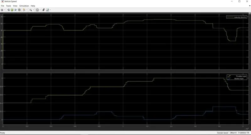
From the above Vehicle Speed plot, we can observe that by increasing the throttle input value, it will increase the Velocity and by increasing the brake input value it will decrease the Velocity.

CVT Shaft Speed Plot:

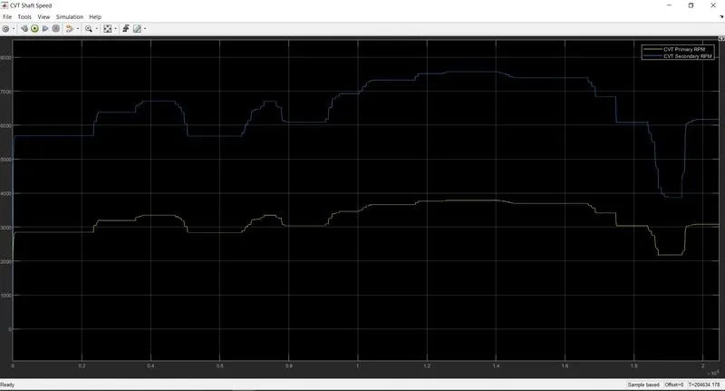
From the above CV Shaft Speed plot, we can observe that by increasing the throttle input value, it will increase the RPM of the Primary & Secondary Pulley and by increasing the brake input value it will decrease the RPM of the Primary & Secondary Pulley.

Engine Speed Plot:

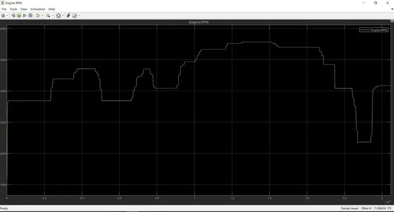
From the above Engine Speed plot, we can observe that by increasing the throttle input value, it will increase the Engine Speed and by increasing the brake input value it will decrease the Engine Speed.

CONCLUSION:

Hence, the System level Simulation of an BAJA All-terrain vehicle for open and closed loop system, Without Using Look Up Table and by Using Look Up Table has been carried out and technical report for the model has been prepared and Output Results are plotted.

REFERENCES:

https://www.caranddriver.com/research/a30822055/what-is-a-cvt-transmission