Project

Aim: To perform a system-level simulation of an all-terrain vehicle.

Objectives:

1. Carry out a system-level simulation of an all-terrain vehicle in open-loop and closed-loop conditions.
2. Analyze the results by varying the inputs.

Model Description:

1. Generic Engine

It represents a system-level model of an IC engine suitable for use at the initial stages of modeling when only basic parameters are available.

Engine inertia was set to 0.008 kg*m^2 and initial velocity was set to 1750 rpm.

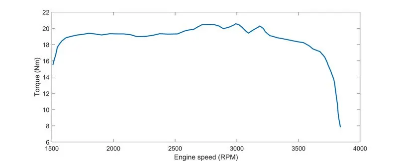
This image shows torque vs engine speed graph

From this image, we can say that the torque is not following a certain trend and is varying as the speed is varying. The peak torque of nearly 21 N-m can be achieved at approximately 2980 rpm. This variation of torque depends on various parameters of the engine.

2. CVT - subsystem

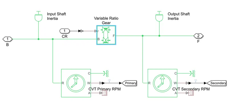
It mainly consists of variable ratio gear, motion sensors, and shaft inertia.

Variable ratio transmission represents variable ratio gearbox. The physical signal input 'r' represents the ratio of input to output angular shaft velocities.

The ideal rotational sensor measures angular velocity and it does not account for any kind of losses.

3. Vehicle Body

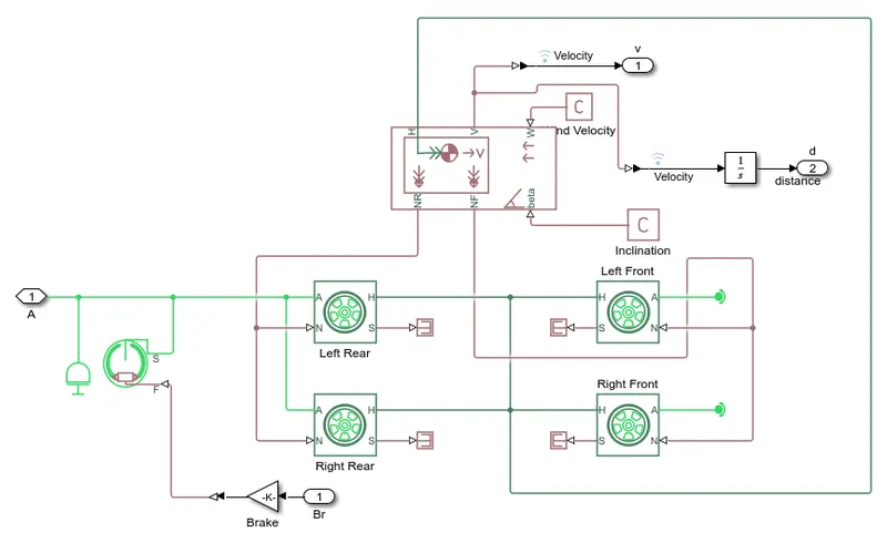
The vehicle body represents a two-axle vehicle body in longitudinal motion. This block accounts for body mass, aerodynamic drag, road incline, and weight distribution between axles due to acceleration and road profile. The vehicle can have the same or a different number of wheels on each axle.

The mass of 250 kg, 2 axles, 0.7 m of CG height above the ground is given to the vehicle body. Also, a drag coefficient of 1.92 is provided as inputs to this block.

The data of 4-wheels such as rated vertical load, rolling radius, inertia, and rolling resistance can be given in this block.

Case-1: Analysis of vehicle in open-loop condition by providing constant throttle and brake inputs

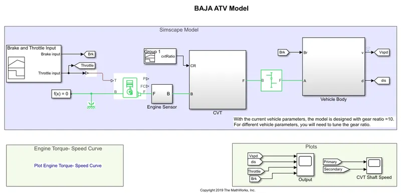
Signal builder is used to creating brake and throttle input signals.

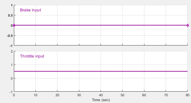
It can be observed that brake input is zero throughout the simulation and throttle input is 0.5 throughout the simulation. These signals are sent to the engine as inputs.

Signal builder is used to get the CVT ratio from the data.

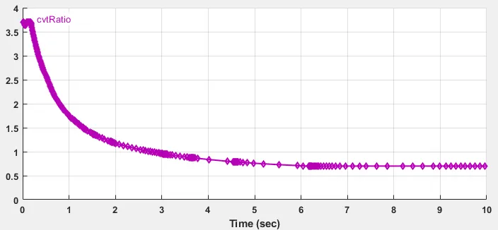
Based on the engine's speed, the CVT ratio is changing.

On performing the analysis with these conditions, the results obtained are:

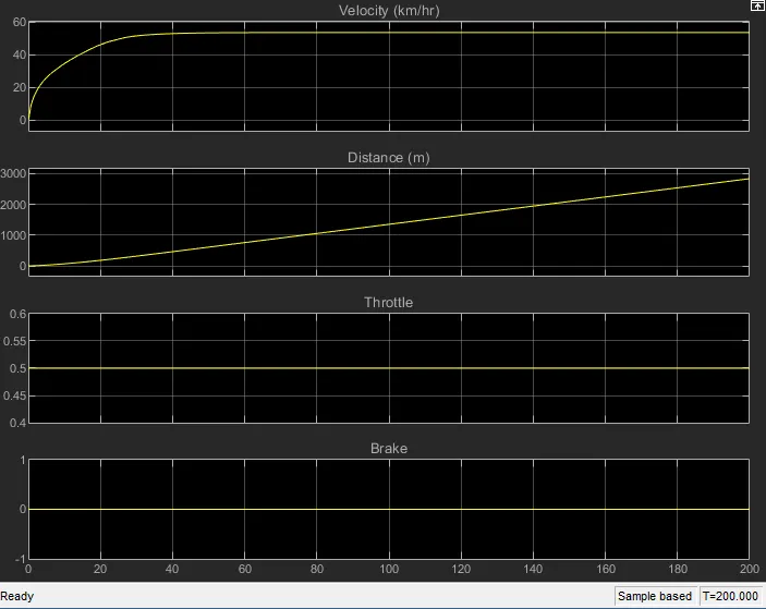
As we know, the brake and throttle remained constant.

The velocity has increased till 40 sec and remained with a constant value of 54 kmph from there. And the distance travelled by the vehicle is gradually increased.

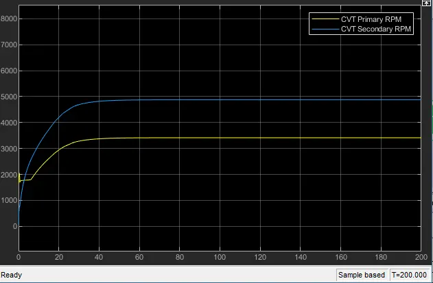
The yellow line indicates CVT primary rpm i.e. speed of the engine and the blue line indicates CVT secondary rpm i.e. output from variable ratio gear.

From the results, we can say that engine has starting speed of nearly 2000 rpm and it decreased for a short period of time and then started increasing. It became constant at nearly 3300 rpm.

CVT secondary rpm has been increasing at faster rates from 0 to 20 sec and then it increased gradually and became constant at nearly 60 sec and 4850 rpm.

Case-2: Analysis of vehicle in open-loop condition by providing varying throttle and brake inputs during the simulation

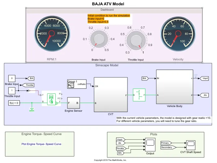
In this condition, we can vary bake and throttle input during the simulation. Knobs are provided for varying the input conditions and the outputs velocity and rpm can be seen in the gauges.

Initial conditions are set to 0 and 0.5 for brake and throttle input. The simulation is made to run for infinite time and we can observe the changes in the gauges by moving the knobs during the time of the simulation.

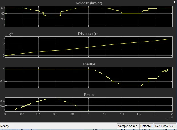
First I have varied the brake input from 0 to 0.5 by keeping the throttle input constant, during that velocity has been reduced to 30 kmph from 60 kmph. And the distance travelled by the vehicle reduced as we applied brakes.

Then I varied the throttle input from 1 to 0.3 by keeping brake input constant, during this, the distance travelled by the vehicle has been reduced with respect to time. And the velocity gradually decreased to 40 kmph.

Case-3: Analysis of vehicle in closed-loop condition by providing constant throttle and brake inputs

In this case, the CVT ratio changes as per vehicle speed. For this we need to use lookup table.

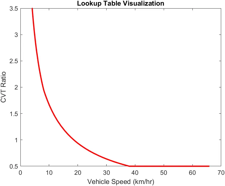
As we see, the CVT ratio is varying from 3.5 at 8 kmph to 0.5 at 38 kmph and it became constant. CVT ratio will be high at lower speeds as the torque required is more at low speeds.

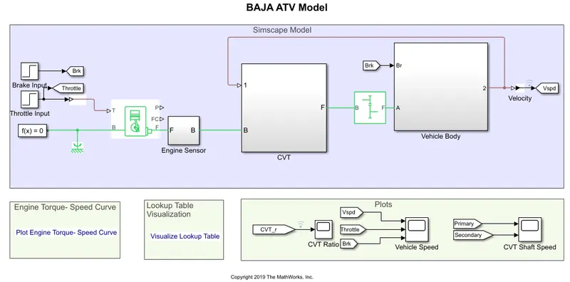Brake and throttle inputs are given as step functions with an initial value of 0 for brake and 0.3 for throttle.

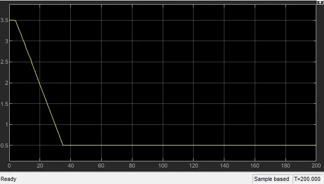
This output of CVT ratio vs time after the simulation. It became constant after 37 sec nearly where the vehicle could have attained maximum speed after 37 sec.

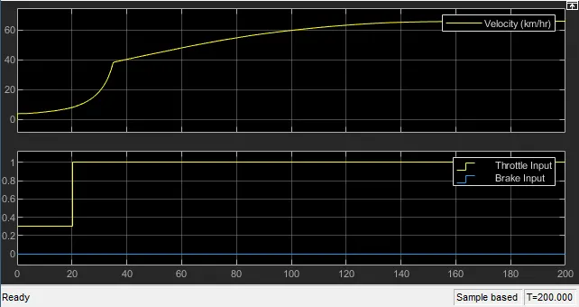
The velocity increased from 5 kmph to 39 kmph in the span of 35 sec and then after it rose gradually with respect to time.

The brake input was kept constant but the throttle increased from 0.3 to 1 in 20 sec and it has kept constant thereafter.

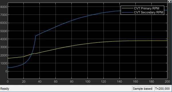
CVT primary rpm is due to the input from the engine. It varies as the throttle and brake inputs are changed.

CVT secondary rpm is due to the vehicle's speed. So, it can be observed that it has a similar trend as that of the vehicle's velocity.

Case-4: Analysis of vehicle in closed-loop condition by providing varying throttle and brake inputs during the simulation

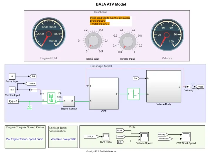
In this condition, we can vary bake and throttle input during the simulation. Knobs are provided for varying the input conditions and the outputs velocity and rpm can be seen in the gauges.

Initial conditions are set to 0 and 0.3 for brake and throttle input. The simulation is made to run for infinite time and we can observe the changes in the gauges by moving the knobs during the time of the simulation.

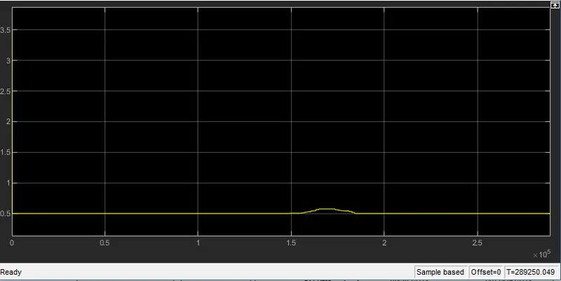
This is how CVT ratio is varying with respect to time. At 0 sec, it changed its value from 3.5 to 0.5. After some time when the brake input is increased, the CVT ratio increased to some extent.

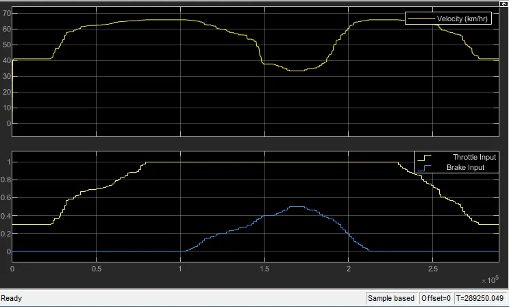
We can observe the change in velocity as the throttle input is increased and the vehicle attained the maximum of 66 kmph with 0 brake input. And it is reduced as the brake input is increased gradually.

The variation of throttle is between 0.3 and 1, variation of brake input is between 0 and 0.5.

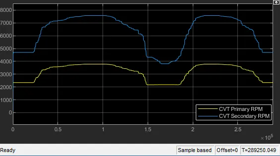
The variation of CVT primary rpm is due to engine throttling and braking.

The variation of CVT secondary rpm is due to the vehicle's speed. So, a similar trend can be observed in between velocity and the CVT secondary rpm.

Conclusion:

• Carried out a system-level simulation of an all-terrain vehicle in open-loop and closed-loop conditions.
• Results were analyzed at 4 different conditions and suitable conclusions were made from those analyses.