Rankine cycle Simulator

Aim: To create a Rankine cycle simulator

Objectives:

• Calculate the state points of the Rankine cycle
• Plot T-S and H-S graphs for a given set of inputs
• To find net work output and back work ratio

Theory:

Steam turbines work on the Rankine cycle. The major parts of the Rankine cycle are the pump, boiler, turbine, and condenser. The Rankine cycle consists of 4 major processes.

Process 1-2: Reversible adiabatic expansion - Turbine

Process 2-3: Constant pressure heat rejection - Condenser

Process 3-4: Reversible adiabatic compression - Pump

Process 4-1: Constant pressure heat supply - Boiler

Formulae:

1. Turbine, Wt = (h1-h2)
2. Condenser, Qr=(h2-h3)
3. Pump, Wp=(h4-h3)
4. Boiler, Qs=(h1-h4)
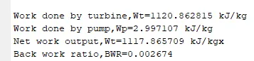
5. Net work, Wnet=Wt-Wp

Wnet=(h1-h2)-(h4-h3)

6. Back work ratio, BWR=Wp/Wt

BWR=(h4-h3)/(h1-h2)

Inputs:

Turbine Inlet temperature = 400° C

Turbine Inlet Pressure = 30 bars

Turbine Outlet Pressure = 0.05 bars = Condenser Inlet Pressure

Main program:

%Program to create Rankine cycle
clear all 
close all
clc

%Processes undergoing in rankine cycle
disp('Process 1-2: Reversible adiabatic expansion - Turbine');
disp('Process 2-3: Constant pressure heat rejection - Condenser');
disp('Process 3-4: Reversible adiabatic compression - Pump');
disp('Process 4-1: Constant pressure heat supply - Boiler');

%Inputs 
T1=input('Enter the turbine inlet temperature:');
p1=input('Enter the turbine inlet pressure:');
p2=input('Enter the condenser inlet pressure:');

%State-1 parameters
h1=XSteam('h_pT',p1,T1);
s1=XSteam('s_pT',p1,T1);

%State-2 parameters
s2=s1;
sf2=XSteam('sL_p',p2);
sg2=XSteam('sV_p',p2);
x2=(s2-sf2)/(sg2-sf2);
hf2=XSteam('hL_p',p2);
hg2=XSteam('hV_p',p2);
h2=hf2+(x2*(hg2-hf2));
T2=XSteam('T_ps',p2,s2);

%State-3 parameters
p3=p2;
T3=T2;
s3=XSteam('sL_p',p3);
h3=XSteam('hL_p',p3);

%State-4 parameters
s4=s3;
p4=p1;
h4=XSteam('h_ps',p4,s4);
Cp=XSteam('Cp_ps',p4,s4);
Cv=XSteam('Cv_ps',p4,s4);
g=Cp/Cv;
T4=T3*((p4/p3)^(g-1)/g);

Tsat=XSteam('Tsat_p',p1);
T5=Tsat;
h5=XSteam('hL_p',p1);
s5=XSteam('sL_p',p1);
T6=Tsat;
h6=XSteam('hV_p',p1);
s6=XSteam('sV_p',p1);

%Work done by the turbine
Wt=h1-h2

%Work done by pump
Wp=h4-h3

%Net work done
Wnet=Wt-Wp

%Back work  ratio
BWR=Wp/Wt

T=linspace(10,500,1000);

%Plotting T-S curve

for i=1:length(T)
    entropy_liquid(i)=XSteam('sL_T',T(i));
    entropy_vapor(i)=XSteam('sV_T',T(i));
end
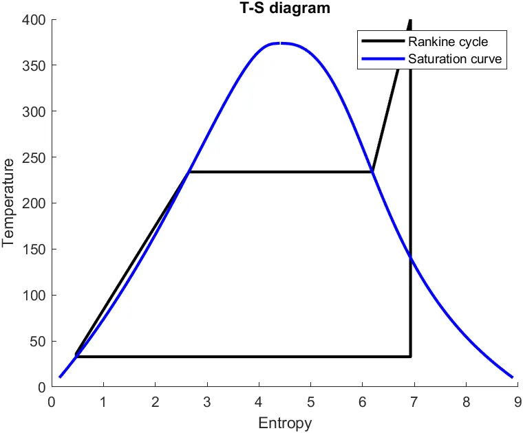
figure(1)
hold on
plot([s1 s2 s3 s4 s5 s6 s1],[T1 T2 T3 T4 T5 T6 T1],'color','k','linewidth',2);
plot(entropy_liquid,T,'color','b','linewidth',2);
plot(entropy_vapor,T,'color','b','linewidth',2);
xlabel('Entropy');
ylabel('Temperature');
title('T-S diagram');
legend('Rankine cycle','Saturation curve');

%Plotting H-S curve

for i=1:length(T)
    enthalpy_liquid(i)=XSteam('hL_T',T(i));
    enthalpy_vapor(i)=XSteam('hV_T',T(i));
    entropy_liquid(i)=XSteam('sL_T',T(i));
    entropy_vapor(i)=XSteam('sV_T',T(i));
end

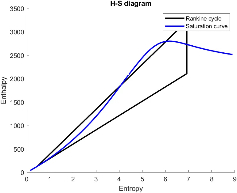
figure(2)
hold on
plot([s1 s2 s3 s4 s1],[h1 h2 h3 h4 h1],'color','k','linewidth',2);
plot(entropy_liquid,enthalpy_liquid,'color','b','linewidth',2);
plot(entropy_vapor,enthalpy_vapor,'color','b','linewidth',2);

xlabel('Entropy');
ylabel('Enthalpy');
title('H-S diagram');
legend('Rankine cycle','Saturation curve');

%Results
fprintf('Results:n')
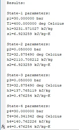
fprintf('nState-1 parameters:np1=%f barnT1=%f deg Celciusnh1=%f kJ/kgns1=%f kJ/kg-Kn',p1,T1,h1,s1)
fprintf('nState-2 parameters:np2=%f barnT2=%f deg Celciusnh2=%f kJ/kgns2=%f kJ/kg-Kn',p2,T2,h2,s2)
fprintf('nState-3 parameters:np3=%f barnT3=%f deg Celciusnh3=%f kJ/kgns3=%f kJ/kg-Kn',p3,T3,h3,s3)
fprintf('nState-4 parameters:np4=%f barnT4=%f deg Celciusnh4=%f kJ/kgns4=%f kJ/kg-Kn',p4,T4,h4,s4)
fprintf('nWork done by turbine,Wt=%f kJ/kgnWork done by pump,Wp=%f kJ/kgnNet work output,Wt=%f kJ/kgxnBack work ratio,BWR=%fn',Wt,Wp,Wnet,BWR)

Explanation:

• Display all the processes undergoing in the Rankine cycle
• T1(turbine inlet temperature), p1(turbine inlet pressure), p2(condenser inlet pressure) are given as the inputs
• Steam data is taken from the 'XSteam' library
• Any parameter can be calculated from the steam table using the inputs given
• For example, h1 can be calculated by using "XSteam('h_pT',p1,T1)" where 'XSteam' is a function and 'h_pT' represents enthalpy as a function of pressure(p1) and temperature(T1)
• Similarly, all the parameters are calculated at every state point
• Also, Tsat is to be extracted from the library
• After calculating all the state point variables, we need to find work done by the turbine, work done by the pump, net work, and back work ratio using appropriate formulae
• Now, we need to plot T-S and H-S diagrams
• Define a temperature range to plot the curves
• 'for' loop is used to plot the curve over a defined teperature range and to get the saturation curves from the 'XSteam' library
• Give appropriate labels, titles, and legends to make the plot more understandable
• After plotting the curves, print the results to the command window using 'fprintf' command

Results:

T-S diagram:

H-S diagram:

Results on command window: