Project – Baja ATV (All Terrain Vehicle) Analysis with CVT using Simulink
Project – Baja ATV (All Terrain Vehicle) Analysis with CVT using Simulink
Aim:
To study the model and analyse the characteristic outcome by performing a simulation using Matlab-Simulink.
Objective:
To study the Baja ATV with Continuously Variable Transmission.
To analyse the technical view in detail for the Baja ATV model with and without the look-up table.
CASE STUDY:
ATV – All Terrain Vehicle:
These vehicles generally represent the off-road vehicles which are suitable for different kinds of terrain even though they are licenced as street-legal motor vehicle in some countries. They have more than two tires (up-to six depending on the requirement) and generally called as “quadricycle” type of vehicles meaning they have handle bar to steer the wheel which is similar to a cycle. These light weight vehicles are defined by American National Standards Institute, runs on low pressure tires and the engine size varies from 49cc to 1000cc depending on the application.
Baja SAE:
Baja SAE challenges engineering students to design and build an off-road vehicle that will survive the severe punishment of rough terrain and in some competitions, water. As in real work situations, these future engineers work together as a team to discover and resolve technical challenges in design, test, and manufacturing, as well as business issues. The most rugged of all the competitions, Baja SAE also gives students the first-hand challenge of pursuing their passion while managing real-life demands and priorities. Each team's goal is to design and build a prototype of an all-weather, rugged, single-seat, off-road recreational vehicle intended for sale to the nonprofessional weekend off-road enthusiast.
SAE International is a global association committed to being the ultimate knowledge source for the engineering profession. By uniting more than 145,000 engineers and technical experts, we drive knowledge and expertise across a broad spectrum of industries.
List of Blocks Used:
| S.NO | Block Name | Function |
| 1 | Constant | To show keep the input constant |
| 2 | Signal builder |
To feed the required input signal. It is used for Brake, Throttle and cvt ratio input. |
| 3 | Solver configuration | To specify the solver parameters before start of simulation |
| 4 | Generic Engine | To run the engine with speed and torque values as input |
| 5 | Mechanical Reference | To make sure all components are clamped to grnd |
| 6 | PS-simulink converter | to convert simscape signal to simulink environment |
| 7 | PS terminator | To terminate any unconnected physical signals in the output side |
| 8 | Simulink-PS converter | converts the simulink signal to simscape environment |
| 9 | PMC_Port |
Physical Modeling Connection Port block for subsystems |
| 10 | Simple gear | To reduce the speed of the engine with pre-define gear ratio |
| 12 | Inertia | Represents solid inertia |
| 13 | Variable ratio transmission | To vary the speed according to the gear ratios |
| 14 | Ideal rotational motion sensor | To sense the rotation of the engine rotor and give the output rpm |
| 15 | Scope | To view graph of the paramerters |
| 16 | Display | To view the calculated engine power |
| 17 | Double shoe brake | To apply brake to the vehicle |
| 18 | PS constant | Generate constant physical signal |
| 19 | Tire | Rotational part(wheel of the vehicle) |
| 20 | Rotational free end | For mechanical tire component |
| 21 | Vehicle body | To represent the vehicle parameters both input and output side |
| 22 | Custom measure Gauges | To measure the brake and throttle input |
| 23 | Knob | To vary the throttle and brake inputs |
| 24 | Look-up table | To insert the CVT values from the workspace |
| 25 | Step | To vary the input value for a defined interval |
Major components used:
Generic Engine:
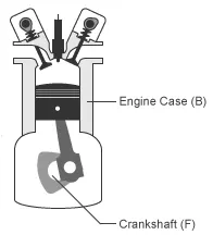
Internal combustion engine, in this type of heat engine the fuel and air mixture ignite and directly, pushes the piston. Diesel and Petrol engines are the best examples of the internal combustion engine. The expansion of the high-temperature and high-pressure gases produced by combustion applies direct force to some component of the engine.
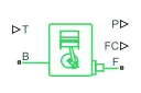
The Generic Engine block represents a general internal combustion engine. This block is a suitable generic engine for spark-ignition and diesel. Speed-power and speed-torque parameterizations are provided. A throttle physical signal input specifies the normalized engine torque. Optional dynamic parameters include crankshaft inertia and response time lag. A physical signal port outputs the engine fuel consumption rate based on the fuel consumption model. It consists of one input port, two output ports and two conserving ports.
Input - T - physical signal port with normalized engine throttle level
Output - P - Instantaneous engine power in W given as physical signal
FC - Fuel consumption rate in Kg/s given as physical signal
Conserve - B - Mechanical rotational conserving port associated with the engine block (physical body) that contains the piston cylinders.
F - Mechanical rotational conserving port associated with the engine crankshaft that transmits the power generated from the combustion process. Typically, you attach a clutch and transmission at this port.
Simple Gear:

The Simple Gear block represents a gearbox that constrains the connected driveline axes of the base gear, B, and the follower gear, F, to corotate with a fixed ratio that you specify. You choose whether the follower axis rotates in the same or opposite direction as the base axis. If they rotate in the same direction, the angular velocity of the follower, ωF, and the angular velocity of the base, ωB, have the same sign. If they rotate in opposite directions, ωF and ωB have opposite signs.
Input - T - Physical signal input port for an external fault trigger.
Conserve - B - Rotational mechanical conserving port associated with the base, or input, shaft.
F - Rotational mechanical conserving port associated with the follower, or output, shaft.
H - Thermal conserving port associated with heat flow. Heat flow affects gear temperature, and therefore, power transmission efficiency.
CVT - Continuously Variable Transmission:
It is one of the type of the transmission developed in late 80's which is commonly used in SUV'S. CVT is similar to automatic transmission but they do not have preset gears, instead the gear ratios are instantly changing and adjusting according to the driving conditions and styles. Hence the drivers don't experience hard shift point in CVT which is why it is called shiftless or single-speed transmission.
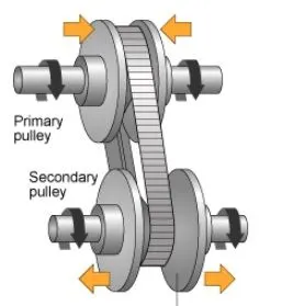
Two half cone shaped pulleys, both move together and apart, connected to chain or V-belt. The belt cross-section rides higher on one pulley, rides lower on the opposite pulley. One side of the pulley is connected to the transmission and other is connected to the engine. The gear ratios seamlessly change moves one pulley together and other far apart. On the whole the CVT consists of belt, a driven pulley system, torque pulley. The main advantage of using CVT is that improves the economy of the fuel, light weight and thus takes less space in the car, has endlessgear shifts and hence can be gas powered. Only few resources are required to build and repair. Driving uphill with CVT instantly shifts to right gear ratio.
The components used to build the CVT in simulink are:
1. Inertia:

The Inertia block represents an ideal mechanical translational inertia. By default, the block has one mechanical translational conserving port. The block positive direction is from its port to the reference point. This means that the inertia torque is positive if inertia is accelerated in the positive direction.
Conserve - I - Mechanical rotational conserving port that connects the inertia to the physical network.
J - Graphical port.
2. Variable Ratio Transmission:

The Variable Ratio Transmission block represents a gearbox that dynamically transfers motion and torque between the two connected driveshaft axes, base and follower.
Conserve - B - Rotational conserving port that represents the base driveshaft.
F - Rotational conserving port that represents the follower driveshaft.
You specify the unitless variable gear ratio gFB(t) as a function of time at the physical signal input at port r. If the signal value becomes zero or negative, the simulation stops with an error.
3. Ideal rotational motion sensor:

The Ideal Rotational Motion Sensor block represents an ideal mechanical rotational motion sensor, that is, a device that converts an across variable measured between two mechanical rotational nodes into a control signal proportional to angular velocity or angle. You can specify the initial angular position (offset) as a block parameter. The sensor is ideal since it does not account for inertia, friction, delays, energy consumption, and so on. Connections R and C are mechanical rotational conserving ports that connect the block to the nodes whose motion is being monitored. Connections W and A are physical signal output ports for velocity and angular displacement, respectively. The block positive direction is from port R to port C.
Vehicle Body:
Vehicle body is the main supporting structure of a vehicle, to which all other components are attached. Truck uses a separate frame as chassis. The vehicle body is designed to carry goods or passengers. Depending on the purpose (trucks, passengers, cargo-passenger, special) and construction (skeleton, half-skeleton, non-skeleton) they change accordingly.
The major components used in vehicle body are:
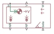
The Vehicle Body block represents a two-axle vehicle body in longitudinal motion. The vehicle can have the same or a different number of wheels on each axle. The vehicle wheels are assumed identical in size. The vehicle can also have acentre of gravity (CG) that is at or below the plane of travel. The block accounts for body mass, aerodynamic drag, road incline, and weight distribution between axles due to acceleration and road profile. Optionally include pitch and suspension dynamics. The vehicle moves only horizontal or parallel to the ground. The block has an option to include an externally-defined mass and an externally-defined inertia. The mass, inertia, andcentre of gravity of the vehicle body can vary over the course of simulation in response to system changes.
Input - W - Physical signal input port for headwind speed
beta - Physical signal input port for road incline angle
CG - Physical signal input port for thecentre of gravity, in m, of the externally-defined mass relative to the CG of the vehicle body.
NR - Physical signal output port for normal force on the rear axle. Wheel forces are considered positive if acting downwards.
Conserve - H - Conserving port associated with the horizontal motion of the vehicle body. Connect tire traction motion to this port.
2. Double brake shoe:

The Double-Shoe Brake block represents a frictional brake with two pivoted rigid shoes that press against a rotating drum to produce a braking action. The rigid shoes sit inside or outside the rotating drum in a diametrically opposed configuration. A positive actuating force causes the rigid shoes to press against the rotating drum. Viscous and contact friction between the drum and the rigid shoe surfaces cause the rotating drum to decelerate.
Input - F - Physical signal input port associated with the applied actuating force.
Conserve - S - Physical signal input port associated with the applied actuating force.
3. Tire:

Tire is the rolling part that is connected to the vehicle body which acts according to the power input given to the axle. This model consists of two front axle and two rear axle tires each.
Input - N - Physical signal input port associated with the normal force acting on the tire. The normal force is positive if it acts downward on the tire
Output - S - Physical signal output port associated with the relative slip between the tire and road.
Conserve - A - Mechanical rotational port associated with the axle that the tire sits on.
H - Mechanical translational port associated with the wheel hub that transmits the thrust generated by the tire to the remainder of the vehicle.
MODEL-1
BAJA ATV MODEL WITHOUT DASHBOARD
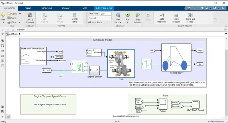
This model consists of three major subsystems namely the engine sensor, CVT and the vehicle body.
Sequence flow:
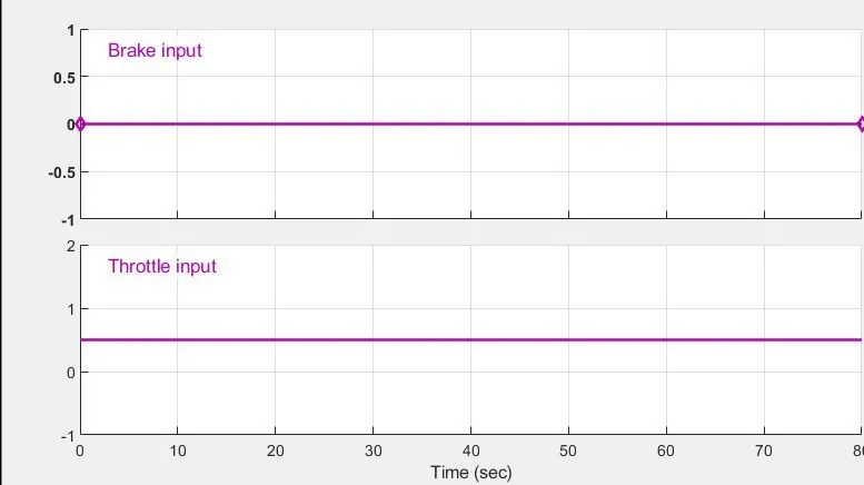
The throttle and brake are the two inputs given to the generic engine. The throttle of 0.5 is given for a period of 80 seconds and hence the brake remains zero during this time period.
These inputs are given to the engine in this case it is a generic engine. Certain engine parameters are required for the efficient working of the atv hence those are specified below.
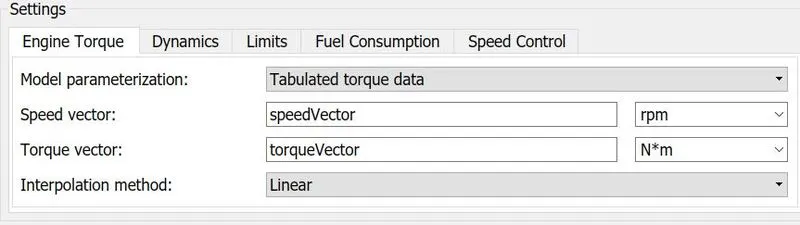
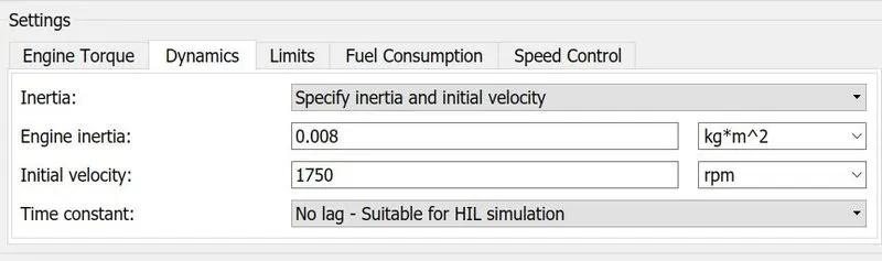
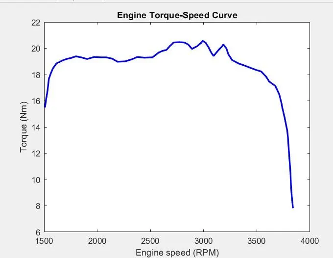
The values of speedVector and torqueVector are defined in the matlab workspace. The data for those two parametersare taken from the engine speed Vs Torque graph which is taken with the help of grabit which is one of the functions of matlab and the collected data can be converted into the desired interpretable format (into excel).
Now the output from the engine is given to ideal rotational motion sensor (here as RPM sensor) which measures the RPM of the engine and the output is obtained in the graphical form using the scope. Any other physical signals obtained at the output is terminated by the PS Terminator.
Engine Sensor
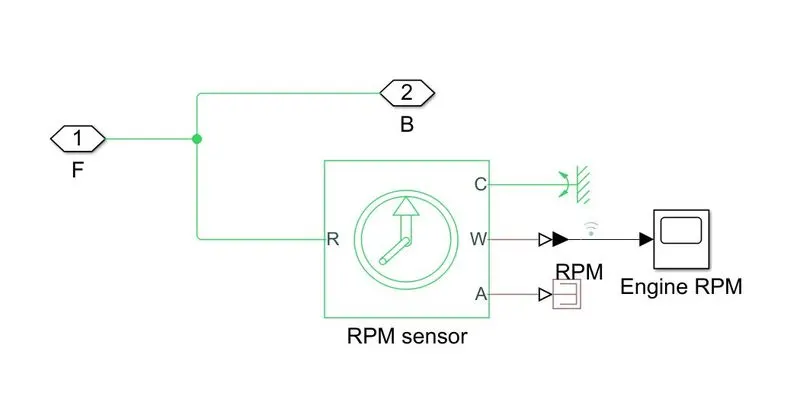
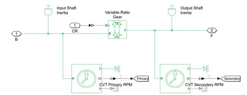
The output of the sensor is connected to the input shaft of the transmission system which is shown as the primary shaft of the CVT. Since the CVT changes seamlessly with its gear ratios, the input for the CVT as per the requirement for an ATV vehicle is given with the help of the signal builder, Inport block and simulink PS- converter (given to 'r') to the Variable ratio transmission block.
INput CVT,
Similar to the input side, the output also consist of an inertia and rotational sensor to measure the secondary RPM.
CVT Transmission
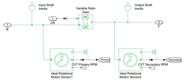
The inertia is defined for this model and have their initial values to begin with. The inertia is calculated for the input and output using,
Input Inertia = `m1*(((18.6e-2)/2)^2+((2.5e-2)/2)^2)/2`
Output Inertia = `m2*(((19.8e-2)/2)^2+((1.9e-2)/2)^2)/2`
The rotational velocity for the input inertia at the beginning is 2500 rpm and for the output is zero. The priority for the input is none but for the output inertia, it is high. Both are measure in `kg*m^2`.
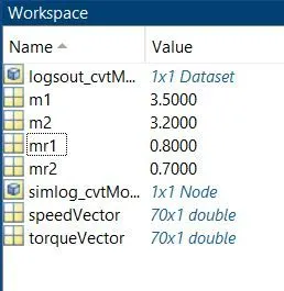
The input inertia m1 and the output inertia m2 are defined in the workspace and their values are 3.5Kg and 3.2Kgrespectively. Using the formulae given above their masses are calculated.
As stated earlier, One pulley of the CVT is connected to the engine side and the other to the transmission side that is the gear box. This component does not include inertia in its model and the output shaft direction is same as the input side. The gear ratio is defined as 10.
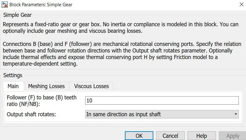
And at the output end the gear box is connected to the vehicle body. In this case the vehicle rear is connected to the gear box.
The vehicle body
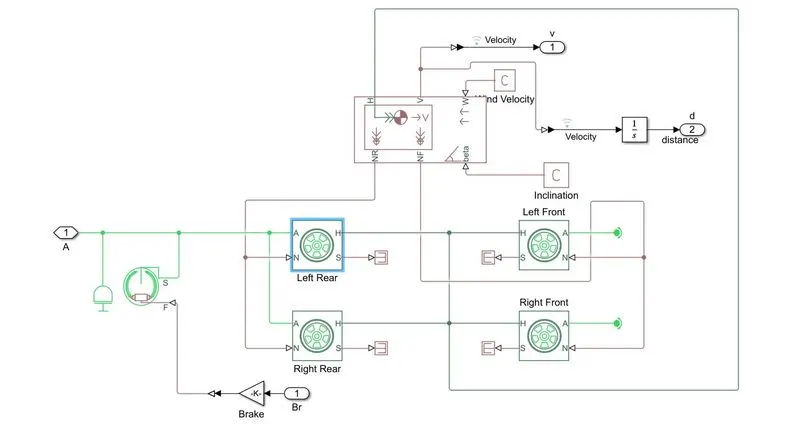
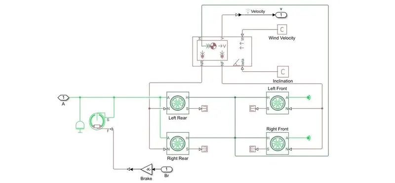
The baja ATV system model shown here is a real-wheel-drive system and hence the gear box is connected to the rear wheels. Also a double shoe brake is connected to the rear side. Two shoes are attached to the drum on the left and right side respectively these eliminates the unbalance created by the normal reactions in the drum and the shaft.
All the elements are connected to the vehicle body block and the parameters of each elements are stated in the vehicle body block as given below:
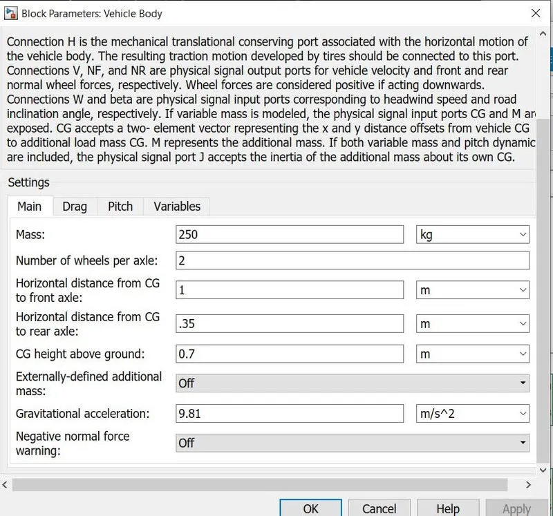
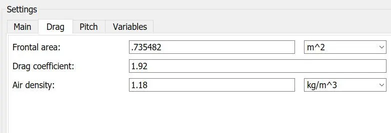
The remaining parameters are not considered or taken as 0 for this model. The vehicle body has only the velocity port as the output. From this port we can get the speed of the vehicle but we also need to know the distance travelled by the vehicle, hence an integer block is connected to the V port to get the distance output.
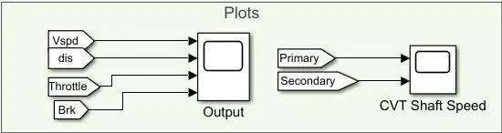
Finally all the outputs are mapped to the scope blocks with the help of the goto tag. The goto block help to get the output from the subsystems. Then the from tag is used to plot those parameters obtained from the goto tag to the scope as shown below.
OUTPUT:
a. The baja ATV model with CVT (without dashboard) where the inputs are given to the engine from the plot (engine torque Vs speed curve) and the other parameters input by the signal builder. As shown in the previous output diagram the output scope is mapped to Vspd(velocity), distance, throttle and brake. The output for the following parameters is shown below.
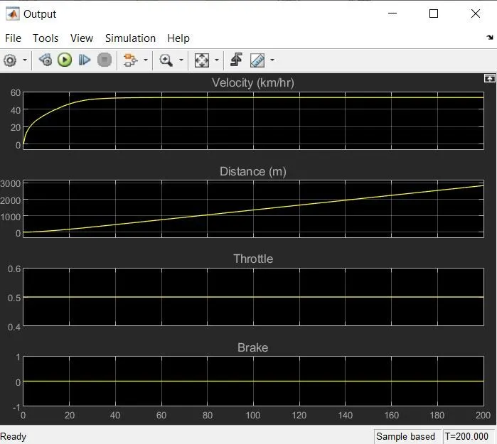
The input given for the brake and the throttle in the signal builder was 0 and 0.5 respectively since when the throttle is pressed the brake is not in use. Hence the output is also the same as input.
b. The CVT primary and secondary outputs are shown below.
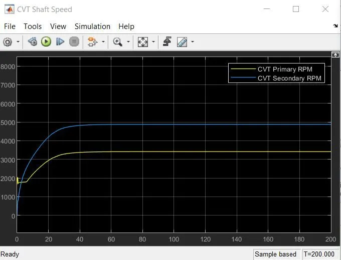
With respect to the input CVT ratio the primary rpm increases, the secondary rpm also increases correspondingly.
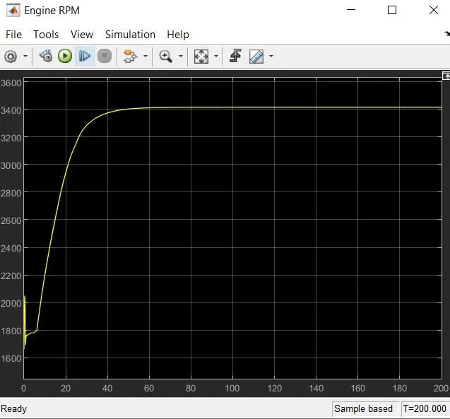
c. The engine RPM is obtained from the engine sensor subsystem.
MODEL-2
BAJA ATV MODEL WITH CVT AND DASHBOARD:
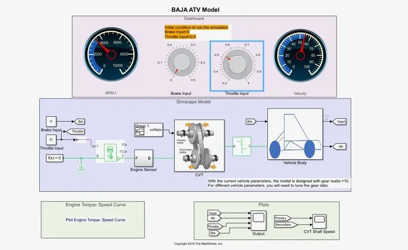
The only change between the model-1 and model-2 is, Baja ATV Model with CVT system where the input to the engine is varied using the knob and then given to the constant block, instead of fixed input given by the signal builder block. The CVT ratio is given using signal builder same as the model-1.
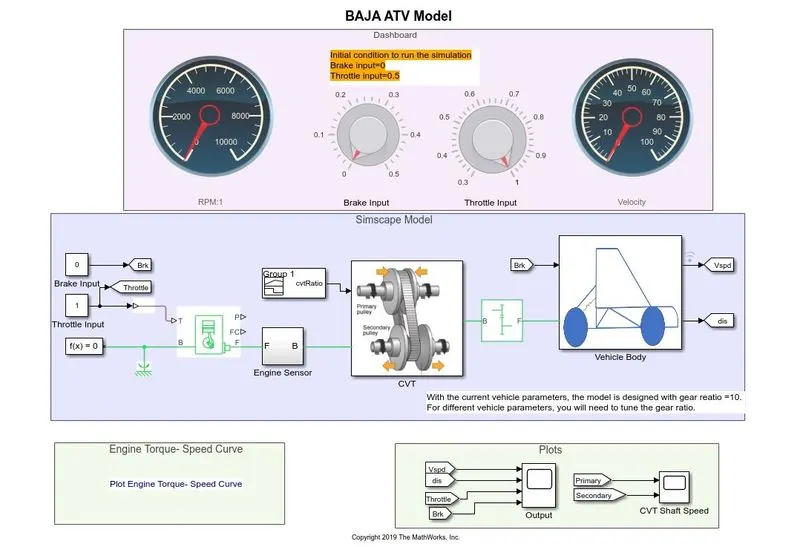
In this model we can change the throttle and brake input to the system by the knob given in the dashboard. The simulation is run for infinity time period so the input brake and throttle is changed during the simulation period and output can be visualized from the scope output. Through this we can learn the real-time effect on the system based on the varying input given.
Two circular gauges, one connected to the RPM of the engine and other to the velocity of the vehicle. The variation is pointed by the movement of the needle in those gauges.
OUTPUT:
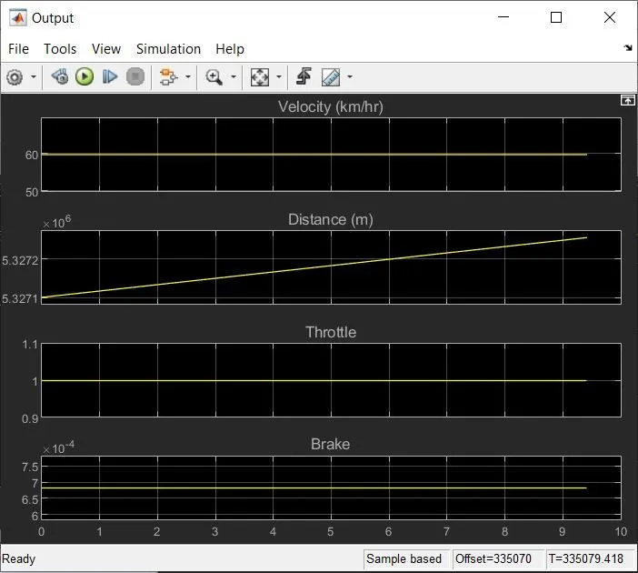
a. Similar to the model-1 we obtain three graphs. The brake and the throttle are controlled by the knob and the cvt ratio is given by the signal builder block. The output for the Vspd(velocity), distance, throttle and brake is shown below. The curve obtained is based on the varied throttle and brake input.
b. Graph for primary and secondary pulleys RPM of CVT:
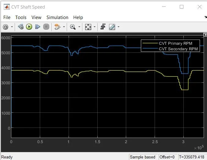
As seen the secondary pulley rpm increases or decreases with respect to the primary pully rpm and the corresponding CVT ratios.
c. Graph for Engine RPM:
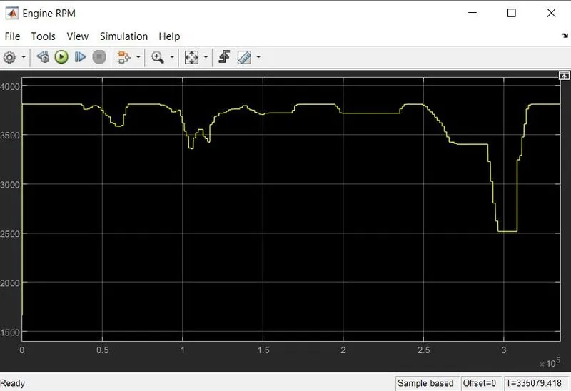
The rpm of the engine changes according to the throttle input.
MODEL-3
Baja ATV model with feedback as input CVT ratio
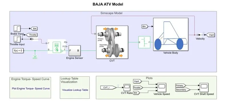
Sequence flow:
In this model, the input for the brake and throttle are given as step signal and there values are defined according to the model requirements as shown below:
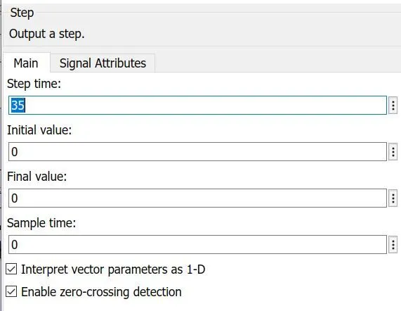
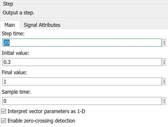
In the above pictures, the values at the left represents the input values of the brake and the values to the right represents the input of the throttle. The throttle is given to the generic engine as the input. Certain engine parameters are required for the efficient working of the atv hence those are specified below.
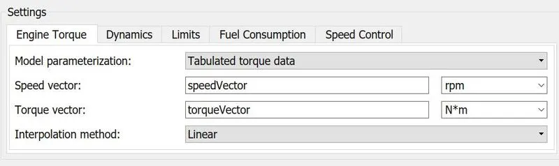
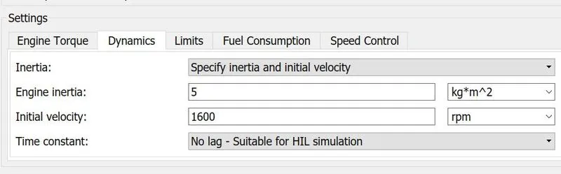
The values of speedVector and torqueVector are defined in the matlab workspace. The data for those two parametersare taken from the engine speed Vs Torque graph which is taken with the help of grabit which is one of the functions of matlab and the collected data can be converted into the desired interpretable format (into excel).
Now the output from the engine is given to ideal rotational motion sensor (here as RPM sensor, an element of the engine sensor subsystem) which measures the RPM of the engine and the output is obtained in the graphical form using the scope. Any other physical signals obtained at the output is terminated by the PS Terminator.
There is no changes in the engine sensor of this model, the same is perceived from model-1 and model-2. The output of the sensor is connected to the input shaft of the transmission system which is shown as the primary shaft of the CVT. 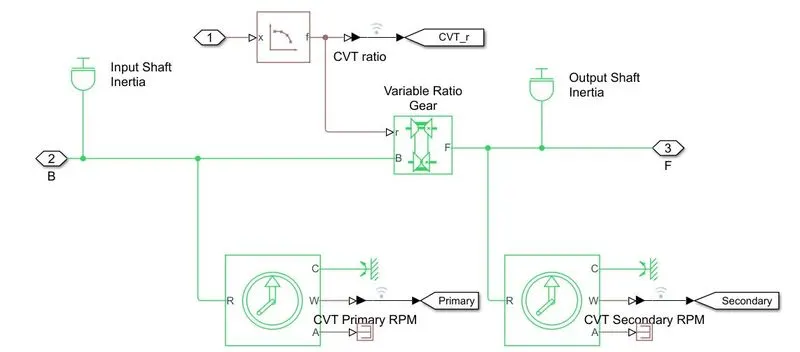
The input for the CVT ratio is given by the look-up table which obtains the input value from the velocity output of the vehicle body block. This forms the feedback loop. Hence the model is called a closed loop model where the instantaneous values are fedback to the input.
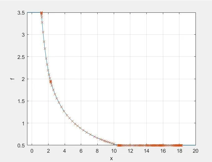
The values considered as the input in the look up table should be in ascending or descending order but the time interval can be non-uniform. Here the vehicle velocity is considered as the input in descending manner.
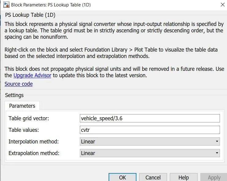
The values plotted in the 1-D lookup table is based on the conditions given in the parameter input box. Here the input to the CVT ratio is vehicle_speed/3.6. Each value is simplified and then fed to the table to form the input. The values obtained after simplification is stored in the variable name cvtr which is the final input given to the 'r' port of the variable ratio transmission block.
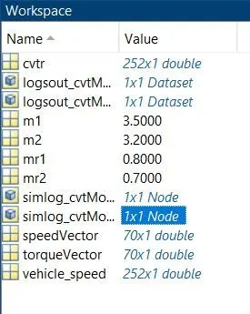
These values are defined in the matlab workspace.
The inertia is defined for this model and have their initial values to begin with. The inertia is calculated for the input and output using,
Input Inertia = `m1*(((18.6e-2)/2)^2+((2.5e-2)/2)^2)/2`
Output Inertia = `m2*(((19.8e-2)/2)^2+((1.9e-2)/2)^2)/2`
The rotational velocity for the input inertia at the beginning is 2500 rpm and for the output is zero. The priority for the input is none but for the output inertia, it is high. Both are measure in `kg*m^2`.
The input inertia m1 and the output inertia m2 are defined in the workspace and their values are 3.5Kg and 3.2Kgrespectively. Using the formulae given above their masses are calculated.
As stated earlier, One pulley of the CVT is connected to the engine side and the other to the transmission side that is the gear box. This component does not include inertia in its model and the output shaft direction is same as the input side. The gear ratio is defined as 12. And at the output end the gear box is connected to the vehicle body. In this case the vehicle rear is connected to the gear box.
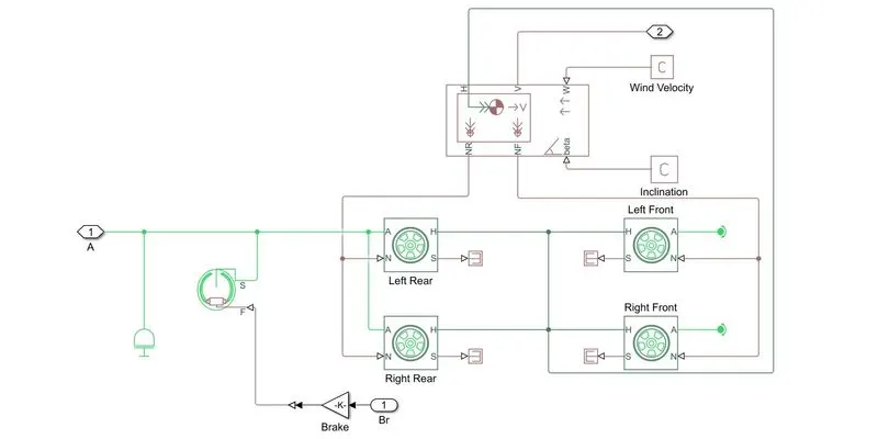
The baja ATV system model shown here is a real-wheel-drive system and hence the gear box is connected to the rear wheels. Also a double shoe brake is connected to the rear side. Two shoes are attached to the drum on the left and right side respectively these eliminates the unbalance created by the normal reactions in the drum and the shaft.
All the elements are connected to the vehicle body block and the parameters of each elements are stated in the vehicle body block as given below:
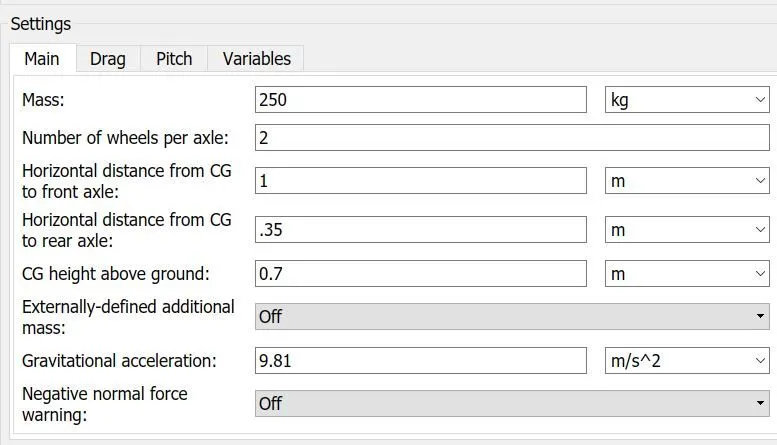
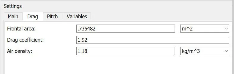
The remaining parameters are not considered or taken as 0 for this model. The vehicle body has only the velocity port as the output. From this port we can get the speed of the vehicle but we also need to know the distance travelled by the vehicle, hence an integer block is connected to the V port to get the distance output.
Finally all the outputs are mapped to the scope blocks with the help of the goto tag. The goto block help to get the output from the subsystems. Then the from tag is used to plot those parameters obtained from the goto tag to the scope.
OUTPUT:
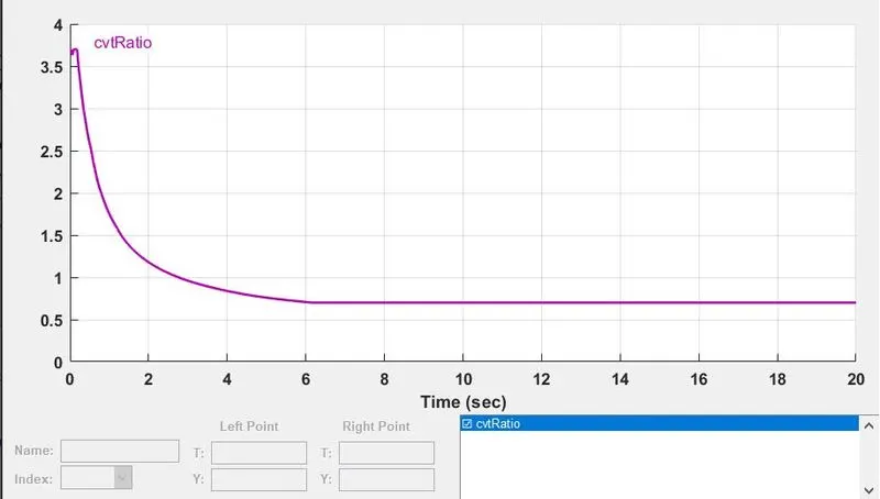
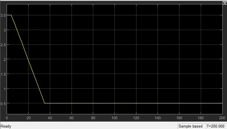
a. Graph for the CVT ratio. AS shown in the input loop-up table the corresponding output for the values of 'cvtr' is plotted in this graph below:
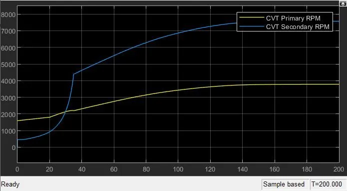
b.The CVT primary and secondary outputs are shown below.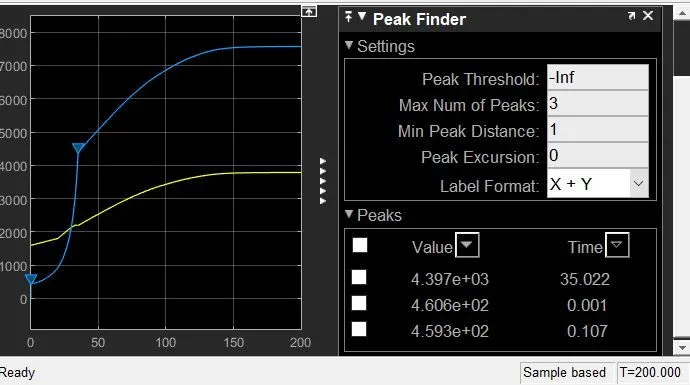
With respect to the input CVT ratio the primary rpm increases, the secondary rpm also increases correspondingly.
c. Graph for the velocity,throttle and brake. The output for the following parameters is shown below.
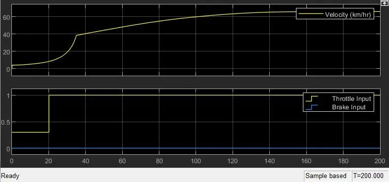
The input given for the brake and the throttle in the step was 0 and 1 respectively since when the throttle is pressed the brake is not in use. Hence the output is also the same as input.
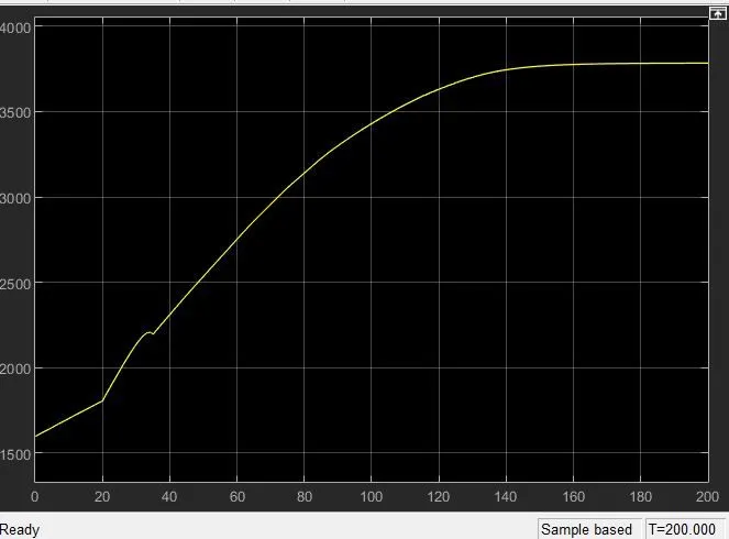
d. Graph for the engine RPM:
MODEL-4
Baja ATV model with feedback as input CVT ratio with dashboard
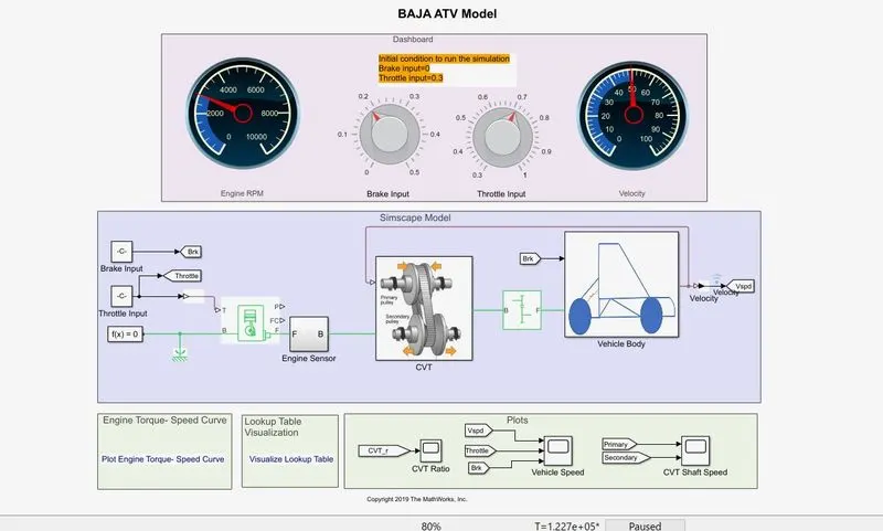
a. This model is same as the previous model-3 except that the input for the brake and the throttle is given by the varying the knob given in the dashboard. The knob and the constant blocks are linked.
b. The simulation time period is defined as infinity so that the input can be varied during the simulation and the varied input can be analysed in the output graphs.
c. Two circular gauges, one representing the engine rpm and the other represents the variation in the velocity of the vehicle. The values displayed in the above picture is in respect to the input values of the throttle and brake given using the knob.
OUTPUT:
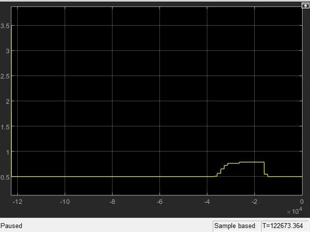
a.Graph for the CVT ratio. AS shown in the input loop-up table the corresponding output for the values of 'cvtr' is plotted in this graph below:
b.The CVT primary and secondary outputs are shown below.
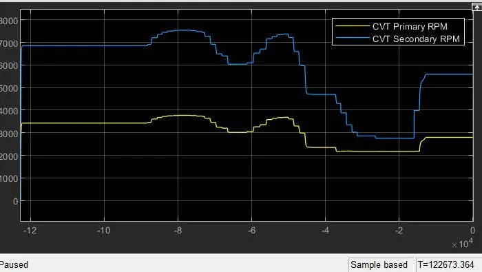
With respect to the input CVT ratio the primary rpm increases, the secondary rpm also increases correspondingly.
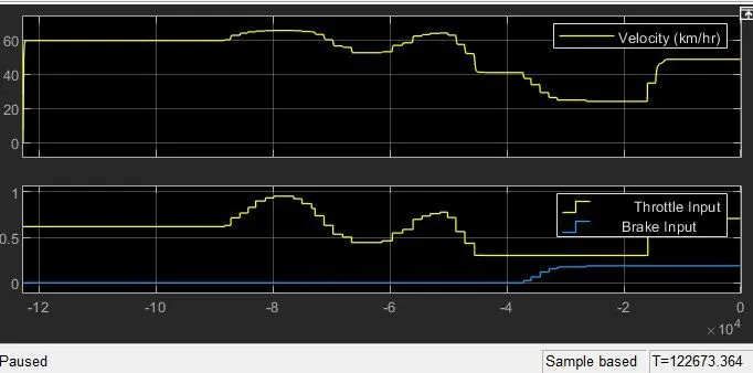
c. Graph for the velocity,throttle and brake. The output for the following parameters is shown below.
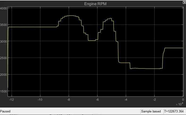
d. Graph for the engine RPM:
MODEL-5
Baja ATV with CVT - output in workspace:
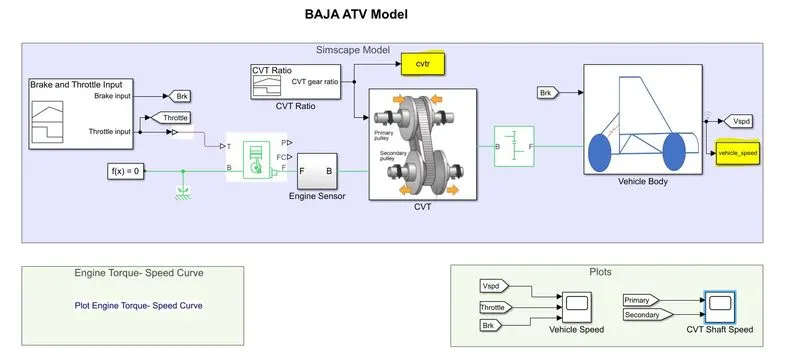
a. This model is similar to the model-1 explained, except that the fixed input given to the CVT ratio by signal builder block differs. And the output of the highlighted blocks 'cvtr' and 'vehicle_speed' is stored in the workspace.
b. All the subsystem are also the same as the model-1:
CVT transmission,
Vehicle body,
The input of the CVT ratio,
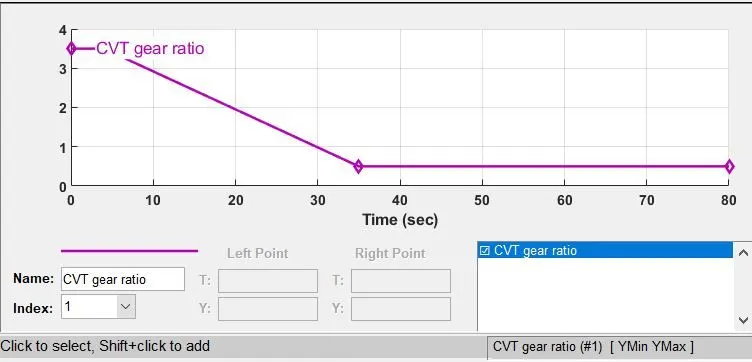
These values are obtained from the graph depicted below
OUTPUT:
a. The outputs "cvtr" and the "vehicle_speed" are shown in the workspace:
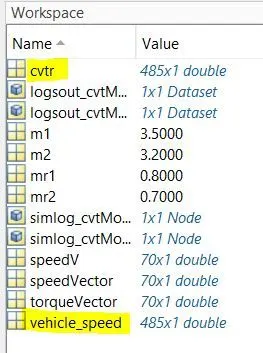
The following commands are executed in the command window for the lookup table to plot the data variables in the workspace

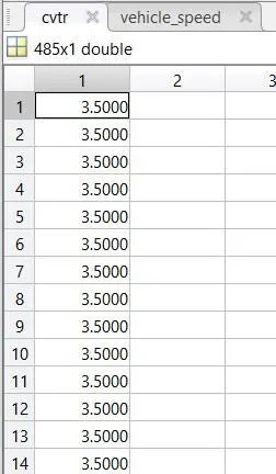
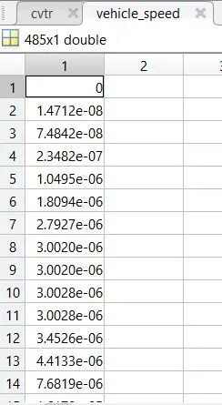
From the image below, to the left is the data output of "cvtr" and to the right is the "vehicle_speed":
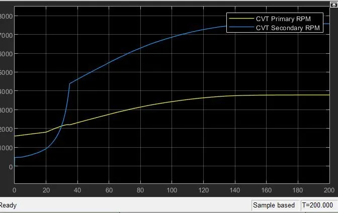
b. The CVT primary and secondary outputs are shown below.
With respect to the input CVT ratio the primary rpm increases, the secondary rpm also increases correspondingly.
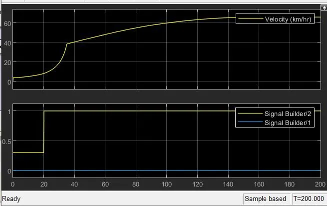
c. Graph for the velocity of the vehicle, brake(signal builder/1) and throttle(signal builder/2):
MODEL-6
Baja ATV with CVT with lookup table input:
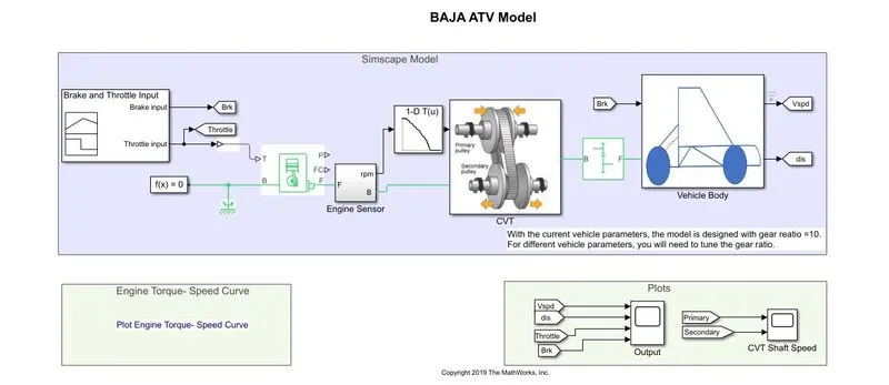
a. This model is similar to the model-5 except the input to the CVT is given as the lookup table where the values are obtained from the rpm of the engine.
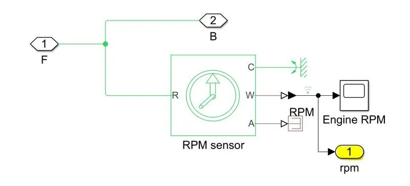
b. The engine sensor which consists of ideal rotational sensor(rpm sensor) is shown below. The output from the sensor is given to the lookup table as highlighted below.
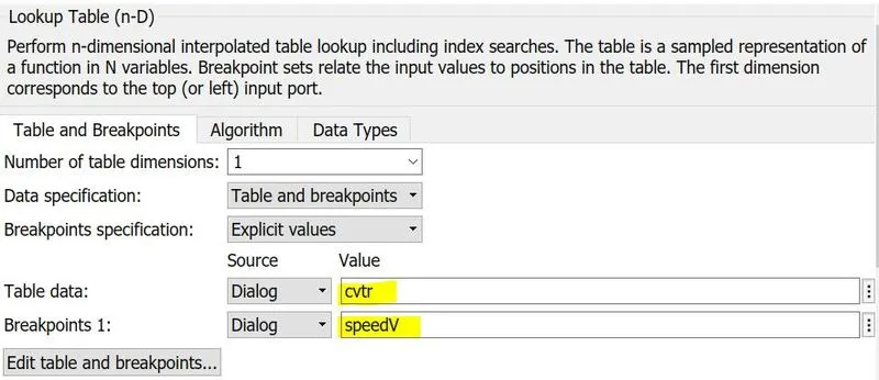
c. LOOKUP TABLE:
The variables "cvtr" and "speedV" are defined in the matlab workspace.
To obtain those variables and to input to our model a matlab script is written to load the variables to the model workspace:

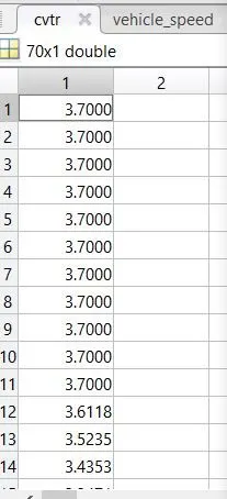
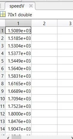
To the left is the cvtr values and to the right is speedV values.
d. CVT:
The output of the sensor is connected to the input shaft of the transmission system which is shown as the primary shaft of the CVT.
The inertia is defined for this model and have their initial values to begin with. The inertia is calculated for the input and output using,
Input Inertia = `m1*(((18.6e-2)/2)^2+((2.5e-2)/2)^2)/2`
Output Inertia = `m2*(((19.8e-2)/2)^2+((1.9e-2)/2)^2)/2`
The rotational velocity for the input inertia at the beginning is 2500 rpm and for the output is zero. The priority for the input is none but for the output inertia, it is high. Both are measure in `kg*m^2`.
The input inertia m1 and the output inertia m2 are defined in the workspace and their values are 3.5Kg and 3.2Kgrespectively. Using the formulae given above their masses are calculated.
e. As stated earlier, One pulley of the CVT is connected to the engine side and the other to the transmission side that is the gear box.
This component does not include inertia in its model and the output shaft direction is same as the input side. The gear ratio is defined as 10. And at the output end the gear box is connected to the vehicle body. In this case the vehicle rear is connected to the gear box.
f. Vehicle body,
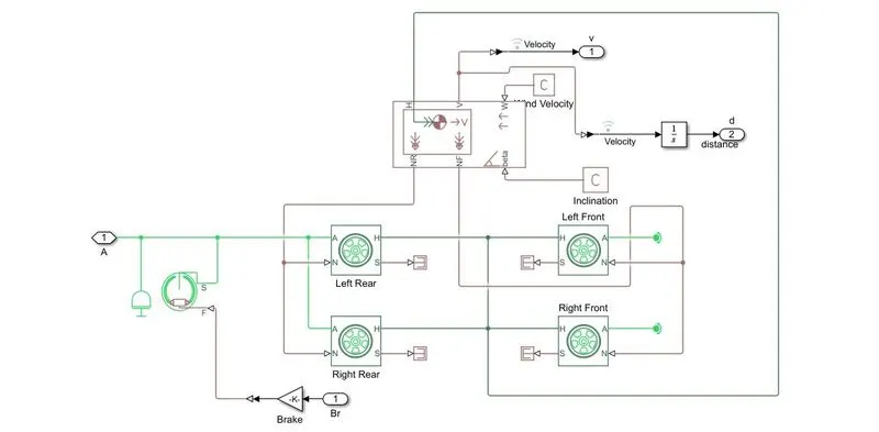
The baja ATV system model shown here is a real-wheel-drive system and hence the gear box is connected to the rear wheels. Also a double shoe brake is connected to the rear side. Two shoes are attached to the drum on the left and right side respectively these eliminates the unbalance created by the normal reactions in the drum and the shaft. All the elements are connected to the vehicle body block and the parameters of each elements are stated in the vehicle body block as given below:
The remaining parameters are not considered or taken as 0 for this model. The vehicle body has only the velocity port as the output. From this port we can get the speed of the vehicle but we also need to know the distance travelled by the vehicle, hence an integer block is connected to the V port to get the distance output.
Finally all the outputs are mapped to the scope blocks with the help of the goto tag. The goto block help to get the output from the subsystems. Then the from tag is used to plot those parameters obtained from the goto tag to the scope.
OUTPUT:
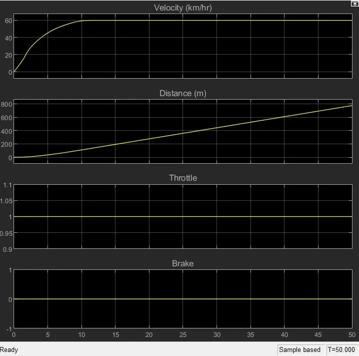
a. As shown in the previous (refer main diagram of model-6) output diagram the output scope is mapped to Vspd(velocity), distance, throttle and brake. The output for the following parameters is shown below.
The input given for the brake and the throttle in the signal builder was 0 and 1 respectively since when the throttle is pressed the brake is not in use. Hence the output is also the same as input.
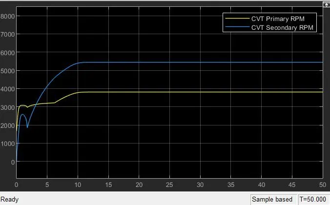
b. The CVT primary and secondary outputs are shown below.
With respect to the input CVT ratio the primary rpm increases, the secondary rpm also increases correspondingly.
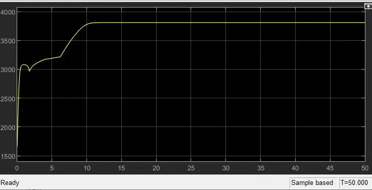
c. The engine RPM is obtained from the engine sensor subsystem.
FINAL VERDICT:
From the above case study, we have analysed 6 models of "BAJA ATV WITH CVT" each differing in the a very few aspects. Also, we have learnt how to incorporate the lookup tables and have analysed their output also. To give the real-time effect we have used lookup tables, dashboard components and feed back models. These help us analyse the system more effectively instead of fixed data input and output. Each model output is studied and also we have learnt the conditions varying each model to given an error free simulation. Thus, simulink makes us get an overall idea of the real world complex model, and analyse the possible errors and outcomes. With the help of this simulation the real world system error can be minimized to a certain level, which makes us produce a cost-effective system and prevent the system from majority of their failures.
REFERENCES:
https://in.mathworks.com/help/physmod/sdl/ref/genericengine.html
https://in.mathworks.com/help/physmod/sdl/ref/simplegear.html?searchHighlight=simple%20gear&s_tid=srchtitle
https://in.mathworks.com/help/physmod/sdl/ref/vehiclebody.html
https://in.mathworks.com/help/physmod/simscape/ref/idealrotationalmotionsensor.html?s_tid=doc_ta