Project 2 Thermal modeling of battery pack
ANSWER:
How Does Temperature Affect the Safety of Lithium-Ion Batteries?
Very low temperatures can produce a reduction in the energy and power capabilities of lithium-ion batteries. High ambient temperatures, however, can contribute to a high internal temperature of the battery — which can also decrease performance and power capabilities.
High ambient temperature is the most important factor that influences UPS battery aging and can cause premature battery failure. Higher temperatures mean a faster chemical reaction inside the battery, which increases water loss and corrosion.
For developing the model we have used the below-given blocks as per the model requirement.
Battery (Table-Based)
Tabulated battery model
- Library:
-
Simscape / Electrical / Sources
Simscape / Battery / Cells

Description
The Battery (Table-Based) block represents a high-fidelity battery model. The block calculates open-circuit voltage as a function of charge level and optional temperature using lookup tables and includes several modeling options:
-
Self-discharge
-
Battery fade
-
Charge dynamics
-
Calendar aging
Use this block to parameterize batteries with complex open-circuit voltage behavior from datasheets or experimental results. For a simpler representation of a battery, see the Battery (Simscape Electrical) block.
The Battery (Table-Based) block has two optional ports that you can expose by setting the corresponding parameters. The extra physical signal port, SOC, outputs the internal state of charge. Use this function to change the load behavior as a function of the state of charge, without the complexity of building a charge state estimator. To expose the SOC port, set the Expose SOC measurement port parameter to Yes in the Main setting.
To expose the thermal port, in the Thermal setting, set the Thermal port parameter to Model. The thermal port represents the battery's thermal mass.
You can also choose different built-in parameterizations for this block. For more information, see the Predefined parameterization section.
The battery equivalent circuit is made up of the fundamental battery model, the self-discharge resistance RSD, the charge dynamics model, and the series resistance R0.
Battery Model
The block calculates the open-circuit voltage or the voltage across the fundamental battery model by interpolation:
v0=v0(SOC,T)
Where:
-
v0 is the open-circuit voltage of the battery. Specify the grid of lookup values using the Open-circuit voltage, V0(SOC, T) parameter if tabulating parameters over temperature, or Open-circuit voltage, V0(SOC) otherwise.
-
SOCis the ratio of current charge to nominal battery capacity specified in the Cell capacity, AH parameter along with the effects of the temperature-dependent fade percentage change in cell capacity, δAH(n, Tfade), specified in the Percentage change in cell capacity, dAH(N, Tfade) parameter. Specify the SOC breakpoints using the Vector of state-of-charge values, SOC parameter. The block estimates the nominal battery capacity based on the number of cycles and the temperature of the battery by interpolating the specified temperature-dependent fade characteristic and the Cell capacity, AH parameter.SOCrepresents the normalized data concerning qnom.For the lookup-table-based fade characteristic option,
qnom(T,n)=(1+δAH(n,Tfade)100)∗AH Ah.
For the equation-based fade characteristic option,
qnom(T,n)=(1+δAH100√nN)∗AH Ah.
Finally,
SOCis obtained from the following equation.SOC(t)=1qnom(T,n)∫(i(t)−Vopen(T,n,t)RSD(T,n))dt
Where:
-
qnom is the cell capacity of the battery. Specify this value using the Cell capacity, AH parameter.
-
N is the reference number of discharge cycles over which you specify the percent change of several battery parameters. Set this value using the Number of discharge cycles, the N parameter.
-
n is the present number of cycles of the battery.
-
δAH is the percentage change in cell capacity of the battery after N discharge cycles.
-
-
T is the battery temperature. Specify the T breakpoints using the Vector of temperatures, T parameter if tabulating the parameters over temperature.
The block also models the series resistance R0 as a function of the state of charge and optional temperature. Specify the grid of lookup values for the series resistance using the Terminal resistance, R0(SOC, T) parameter if tabulating the parameters over temperature, or Terminal resistance, R0(SOC) otherwise.
THESE BATTERIES ARE CONNECTED IN THE SERIES TO PERFORM THE SIMULATION.
Controlled Current Source
The ideal current source is driven by the input signal
Library
Electrical Sources

Description
The Controlled Current Source block represents an ideal current source that is powerful enough to maintain the specified current through it regardless of the voltage across the source.
The output current is I = Is, where Is is the numerical value presented at the physical signal port.
The positive direction of the current flow is indicated by the arrow.
Ports
The block has one physical signal input port and two electrical conserving ports associated with its electrical terminals.
This block has been.
IT IS USED TO CONTROL THE ELECTRIC CURRENT REQUIRED FOR THE MODEL.
Voltage Sensor
- Library:
-
Simscape / Foundation Library / Electrical / Electrical Sensors
Simscape / Electrical / Sensors & Transducers

Description
The Voltage Sensor block represents an ideal voltage sensor, a device that converts voltage measured between two points of an electrical circuit into a physical signal proportional to the voltage.
Use the + and - ports to connect the sensor in parallel with the block (or several blocks) where you want to measure the voltage. Port V outputs the measurement result as a physical signal. Use a PS Simulink Converter block to connect this port to Simulink® blocks, such as Scope or Display.
Ports
Output
V — Voltage, V
physical signal
Conserving
+ — Positive terminal
electrical
- — Negative terminal
electrical
IT IS USED TO MEASURE THE VOLTAGE OF THE MODEL WHICH INCLUDES 10 BATTERIES THAT ARE CONNECTED IN THE SERIES.
Current Sensor
- Library:
-
Simscape / Foundation Library / Electrical / Electrical Sensors
Simscape / Electrical / Sensors & Transducers

Description
The Current Sensor block represents an ideal current sensor, a device that converts current measured in any electrical branch into a physical signal proportional to the current.
Use the + and - ports to connect the sensor in series with the other blocks in the branch where you want to measure the current. Port I outputs the measurement result as a physical signal. Use a PS- Simulink converter block to connect this port to Simulink® blocks, such as Scope or Display.
Ports
Output
I — Current, A Physical signal output port for the electrical current measurement
physical signal
Conserving
+ — Positive terminal
electrical. Electrical conserving port associated with the sensor-positive terminal
- — Negative terminal
electrical. Electrical conserving port associated with the sensor negative terminal.
Conductive Heat Transfer
Heat transfer by conduction
- Library:
-
Simscape / Foundation Library / Thermal / Thermal Elements

Description
The Conductive Heat Transfer block represents heat transfer by conduction between two layers of the same material. For a flat surface, the Fourier law describes the transfer,
Q=k⋅AD(TA−TB),
where:
-
Q is the heat flow.
-
k is the thermal conductivity of the material.
-
A is the area normal to the heat flow direction.
-
D is the distance between layers, that is, the thickness of the material.
-
TA is the temperature of layer A.
-
TB is the temperature of layer B.
Heat conduction through a round pipe wall is
Qcyl=2πk⋅Lln(doutdin)(TA−TB),
where:
-
L is the pipe length.
-
din is the inner diameter.
-
dout is the outer diameter.
You can specify the thermal conductivity by using the Conductivity type parameter:
-
Constant— Thermal conductivity remains constant during simulation. You specify the thermal conductivity by using the Thermal conductivity parameter. -
Variable input— You specify the thermal conductivity using the input physical signal at port K, which can vary during simulation. The Minimum thermal conductivity parameter specifies the lower bound for the physical signal. -
Tabulated data— You specify the thermal conductivity by using a lookup table based on temperature. In this case, thermal conductivity can also vary during simulation.
The Tabulated data option uses the average temperature of the block to find the thermal conductivity. For planar wall geometry, the average temperature is
Tavg=TA+TB2.
For cylindrical wall geometry, the average temperature is
Tavg=(TA−TB)⋅⎛⎜⎜⎝doutdout−din−1ln(doutdin)⎞⎟⎟⎠+TB,
which assumes that TB is at the inside of the cylinder.
A and B are thermal conserving ports associated with the material layers. Because the block's positive direction is from port A to port B, the heat flow is positive if it flows from A to B.
Variables
To set the priority and initial target values for the block variables prior to simulation, use the Initial Targets section in the block dialog box or Property Inspector. For more information, see Set Priority and initial Target for block variables.
Nominal values provide a way to specify the expected magnitude of a variable in a model. Using system scaling based on nominal values increases the simulation's robustness. Nominal values can come from different sources, one of which is the Nominal Values section in the block dialog box or Property Inspector. For more information, see Modify Nominal Values for a Block Variable.
Ports
Input
K — Thermal conductivity control signal, W/(K*m)
physical signal
Conserving
A — Layer A
thermal
B — Layer B
thermal
Parameters
Conductivity type — How to specify thermal conductivity
Constant (default) | Variable input | Tabulated data
Wall geometry — Wall shape for heat conduction
Planar (default) | Cylindrical
Area — Area of heat transfer
1e-4 m^2 (default) | positive scalar
Thickness — Thickness of material
0.1 m (default) | positive scalar
Inner diameter — Inner diameter of the pipe
0.05 m (default) | positive scalar
Outer diameter — Outer diameter of the pipe
0.1 m (default) | positive scalar
Length — Pipe length
1 m (default) | positive scalar
Thermal conductivity — Thermal conductivity of the material
401 W/(K*m) (default) | positive scalar
Minimum thermal conductivity — Lower bound for thermal conductivity
10 W/(K*m) (default) | positive scalar
Thermal conductivity vector — Vector of thermal conductivity values for use in table lookup
[413, 401, 392, 383, 371, 357, 342] W/(K*m) (default) | vector of positive values
Temperature vector — Vector of temperature values for use in table lookup
[200, 273, 400, 600, 800, 1000, 1200] K (default) | strictly increasing vector
Convective Heat Transfer
- Library:
-
Simscape / Foundation Library / Thermal / Thermal Elements

Description
The Convective Heat Transfer block represents heat transfer by convection between two bodies using fluid motion. The Newton law of cooling describes the transfer,
Q=k⋅A⋅(TA−TB),
where:
-
Q is the heat flow.
-
k is the convection heat transfer coefficient.
-
A is the surface area.
-
D is the distance between layers, that is, the thickness of the material.
-
TA and TB are the temperatures of the two bodies.
The heat transfer coefficient, k, can be either constant, which you specify by using the Heat transfer coefficient parameter, or variable, which you specify by using the physical signal at port K.
A and B are thermal conserving ports associated with the points between which the heat transfer by convection takes place. Because the block's positive direction is from port A to port B, the heat flow is positive if it flows from A to B.
Variables
To set the priority and initial target values for the block variables prior to simulation, use the Initial Targets section in the block dialog box or Property Inspector. For more information, see Set Priority and initial Target for block variables.
Nominal values provide a way to specify the expected magnitude of a variable in a model. Using system scaling based on nominal values increases the simulation's robustness. Nominal values can come from different sources, one of which is the Nominal Values section in the block dialog box or Property Inspector. For more information, see Modify Nominal Values for a Block Variable.
Ports
Input
K — Heat transfer coefficient control signal, W/(K*m^2)
physical signal
Conserving
A — Body A
thermal
B — Body B
thermal
Parameters
Convection type — How to specify heat transfer coefficient
Constant (default) | Variable
Area — Area of heat transfer
1e-4 m^2 (default) | positive scalar
Heat transfer coefficient — Convection heat transfer coefficient
20 W/(K*m^2) (default) | positive scalar
Minimum heat transfer coefficient — Lower bound for heat transfer coefficient
1e-3 W/(K*m^2) (default) | positive scalar
Temperature Source
A constant source of thermal energy, characterized by temperature
- Library:
-
Simscape / Foundation Library / Thermal / Thermal Sources

Description
The Temperature Source block represents an ideal source of thermal energy that is powerful enough to maintain a specified temperature at its outlet regardless of the heat flow consumed by the system.
The source generates constant absolute temperature, defined by the Temperature parameter value.
Ports
Conserving
Thermal conserving port associated with the source outlet
A — Source outlet
thermal
Parameters
The constant absolute temperature at the source outlet port.
Temperature — Absolute temperature at source outlet
293.15 K (default)
IT IS USED TO AS A TEMPERATURE SOURCE AT DIFFERENT VALUES
Temperature Sensor
Ideal temperature sensor
Library
Thermal Sensors

Description
The Temperature Sensor block represents an ideal temperature sensor, that is, a device that determines the temperature differential measured between two points without drawing any heat.
Connections A and B are thermal conserving ports that connect to the two points where the temperature is being monitored. Port T is a physical signal port that outputs the temperature differential value.
The block's positive direction is from port A to port B. The measured temperature is determined as T = TA – TB.
Ports
The block has the following ports:
A-
Thermal conserving port associated with the sensor positive probe.
B-
Thermal conserving port associated with the sensor negative probe.
T-
Physical signal output port for temperature.
IT IS USED TO MEASURE THE TEMPERATURE.
- From and Goto blocks
The Goto block passes its input to its corresponding From blocks. The input can be a real- or complex-valued signal or vector of any data type. From and Goto blocks allow you to pass a signal from one block to another without actually connecting them.
The From block accepts a signal from a corresponding Goto block, then passes it as output. The data type of the output is the same as that of the input from the Goto block. From and Goto blocks allow you to pass a signal from one block to another without actually connecting them.
WE BUILT THE BELOW MODEL TO PERFORM THE SIMULATION.
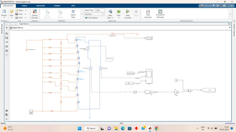
we performed simulations at different temperatures to observe the battery model performance. For 1000 seconds.
RESULT:
CASE 1:
TEMPERATURE AT 293.1K
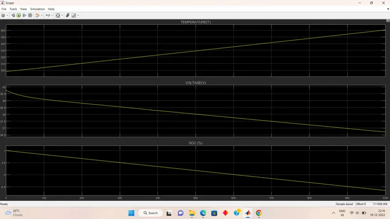
1. In the first plot we can observe temperature is being increased to a maximum of above 360K for the end of the simulation.
2. In the second plot we can observe voltage being decreased as temperature increases for the entire simulation of time.
3. In the third plot we can observe the state of cha also decreases as voltage decreases and temperature increases for the entire simulation of time.
CASE 2:
TEMPERATURE AT 320K :
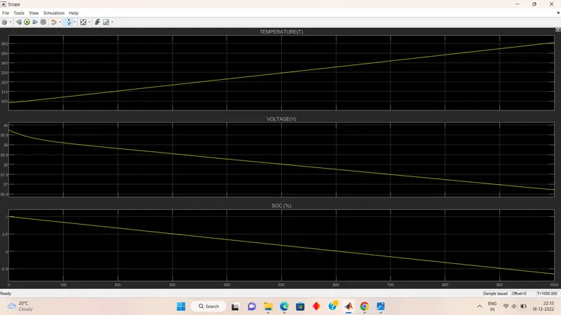
1. In the first plot we can observe temperature is being slightly increased to a maximum of above 362K for the end of the simulation. as the temperature is increased.
2. In the second plot we can observe voltage being decreased as temperature increases for the entire simulation of time.
3. In the third plot we can observe the state of cha also decreases as voltage decreases and temperature increases for the entire simulation of time.
CASE 3:
TEMPERATURE AT 240K :
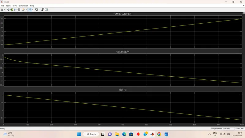
1. In the first plot we can observe temperature is being slightly decreased to below 360K for the end of the simulation. as the temperature is decreased.
2. In the second plot we can observe voltage being decreased as temperature increases for the entire simulation of time.
3. In the third plot we can observe the state of cha also decreases as voltage decreases and temperature increases for the entire simulation of time.