Project 2 Thermal modeling of battery pack

AIM:-

For a 10 cell series lithium ion battery model, simulate the thermal effects and compare life cycle performance at various temperatures, charge & discharge rates using MATLAB.

Theory:-

The performance of lithium-ion batteries is influenced by both operating voltage and temperature. Lithium-ion batteries perform best at specific voltage and temperature ranges; otherwise, irreparable damage to the batteries will result.

When there is an overvoltage, the charging voltage is higher than the tolerable cell voltage, which results in excessive current flows and simultaneously creates two issues.

To prevent thermal problems and enhance performance, the battery temperature should be kept within set temperature ranges. The battery system needs a thermal management system because the temperature range affects battery power and cycle life. At the same time, the temperature distribution needs to be uniform to ensure battery performance and lifetime.

The maximum battery power is reached at temperatures between 20 and 40 degrees centigrade.

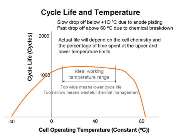
The cycle life goes down slowly below 10 degrees because of anode plating and drops off quickly above 60 degrees centigrade due to the breakdown of electrode materials.

Generally, the temperature must be controlled between 20 degrees to 40 degrees centigrade to ensure performance and cycle life.

Simulink Model:-

Main components and their factors:-

Battery(table-based):

Controlled Current Source:

The block represents an ideal current source that is powerful enough to maintain the specified current through it regardless of the voltage across it. The output current is I = Is, where Is is the numerical value presented at the physical signal port.

Current sensor:

The block represents an ideal current sensor, that is, a device that converts current measured in any electrical branch into a physical signal proportional to the current.Connections + and - are conserving electrical ports through which the sensor is inserted into the circuit. Connection I is a physical signal port that outputs current value.

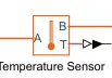
Temperature Sensor:

This block measures temperature in a thermal network. There is no heat flow through the sensor. The physical signal port T reports the temperature difference across the sensor. The measurement is positive when the temperature at port A is greater than the temperature at port B.

Temperature Source:

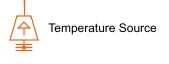
This block represents an ideal energy source in a thermal network that can maintain a constant absolute temperature at the port regardless of the heat flow rate.

Convective heat Transfer:

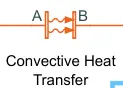
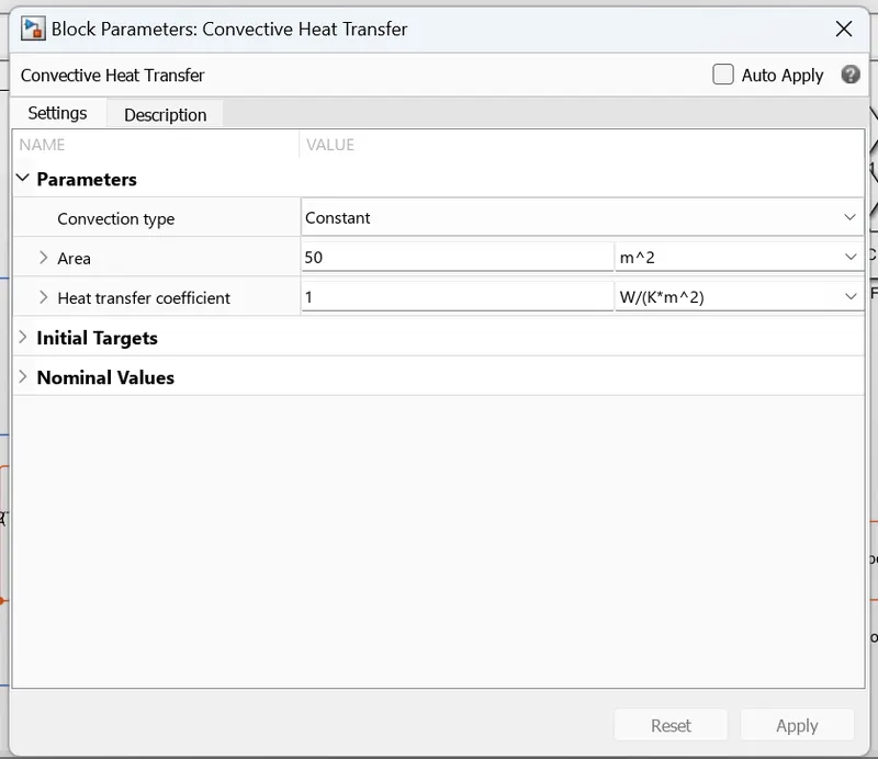
This block models heat transfer in a thermal network by convection due to fluid motion. The rate of heat transfer is proportional to the temperature difference, heat transfer coefficient, and surface area in contact with the fluid.

Voltage Sensor:

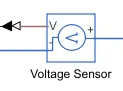
The block represents an ideal voltage sensor, that is, a device that converts voltage measured between any electrical connections into a physical signal proportional to the voltage.Connections + and - are conserving electrical ports through which the sensor is connected to the circuit. Connection V is a physical signal port that outputs voltage value.

Signal Builder:

Scope:

Working on Simulink Model:-

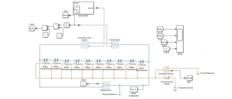
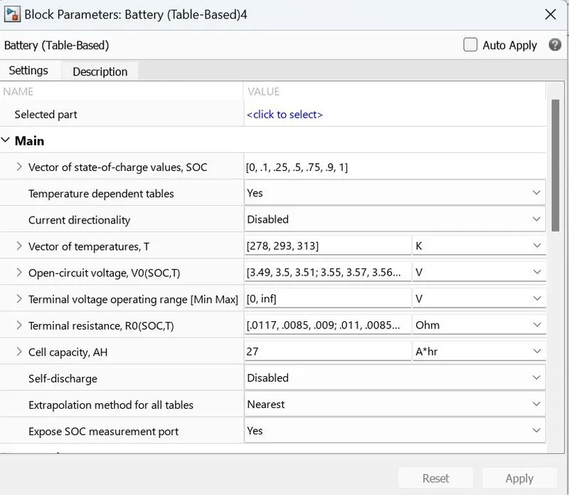
First, we used the table-based battery. Next, we instrumented it, displayed the thermal port, and left the rest of the parameters at their default values. We used default data from Matlab rather than data from a data sheet. Then, using the same design, we connected ten more similar cells in a row. Since the capacity is the same across the pack, the voltage across it is multiplied by 10 instead.
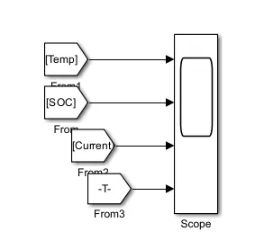
A voltage sensor is now connected to the two transformers, one of which is negative from the first and the other is positive from the last, and a goto block is connected to the voltage sensor via a ps to simulink converter to take the output voltage, while a from block is connected to the scope to receive the voltage signal.
A current sensor is attached to the regulated current source, which is connected to the battery to draw current from it. The current is then connected to the block via a ps to simulink converter, where a from block is present to receive the signal and transmit it to the scope.

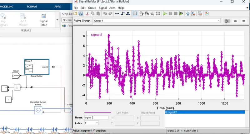
UDDS drive cycle data is employed in the form of current with regard to time and a signal builder is used to provide the input to the controlled current sensor.
In order to enhance the area of contact and as we provide the temperature input to the temperature source block, the temperature source is now linked to the thermal port to provide the external temperature. This connection is made via the convective heat transfer block rather than directly. In order to gauge the battery pack's temperature, a temperature sensor is placed there, and one port is linked to a thermal reference.
The temperature signal is sent from the temperature sensor's output via a ps to simulink converter block and a from block that is linked to the scope.
Finally, a solver configuration and an electrical reference are attached to the model's electrical side for ground.
As the input current is just for the first 1369 seconds, we run the simulation for that length of time because after that, the graph will remain unchanged because no load current is being pulled from it.

Simulation Results:-

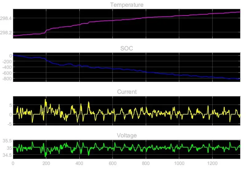
The blocks are all given default values at this place, and the simulation results are shown. Because we utilized it the same way, the current drawing is shown in the first graph. You can see that the greatest value is up to 5 and the smallest value is -5, which represents charging regen braking.
The second graph depicts a SOC that is falling yet linear; depending on whether the current is positive or negative, it is sometimes charging and occasionally discharging.
After running the whole simulation, it is at 0.992, which is about full, starting from 1 which is full charge.
The third graph shows the temperature, which is the default graph for which I made no adjustments. As a result, it rose marginally 
The voltage fluctuation is the final to be discussed. It begins at 34.5 volts and concludes at the same 35 volts throughout time, growing and decreasing as the battery is charged or discharged.

By changing values:-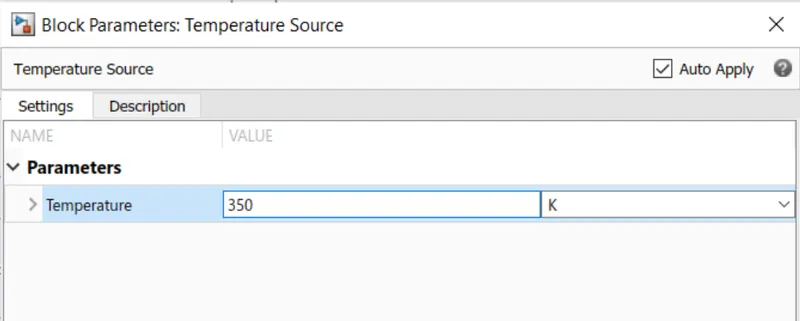

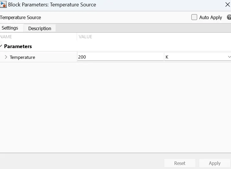
Here from the temperature source, we change the temperature to 350k.

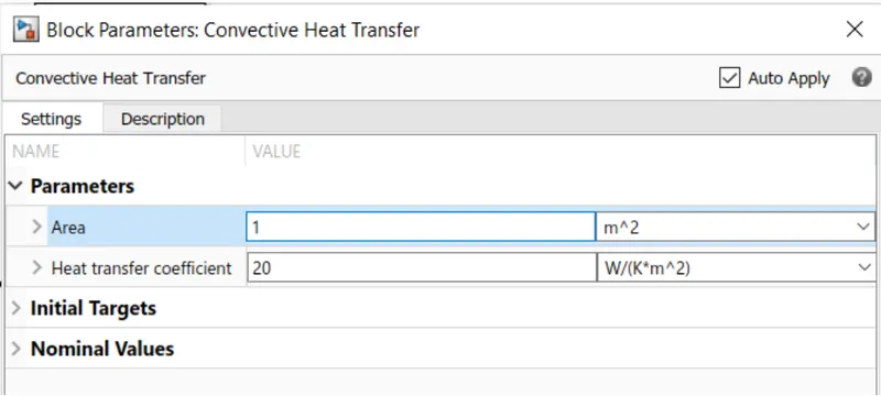
And in convective heat transfer, the area we made from 1e-1 to 1m^2.

let's see the result of the simulation time

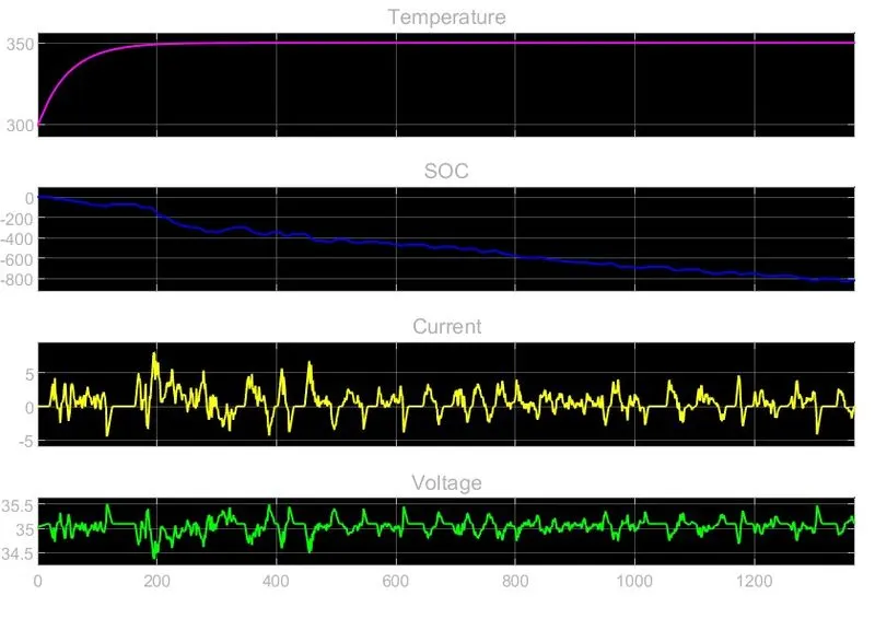
Because we didn't make any changes to the load side, the first graph of current is the same as what we can see here. Similar to the previous graph.
The runtime is so low that we cannot see any differences in the second graph, which represents the social sector.
The first graph, which shows temperature as a function of time, has been altered so that it initially starts at 300, increases to 350, and then remains constant.
So yes, there is a difference between this one and the previous one.
The final graph is a voltage one, which resembles the first one quite a bit.

By changing the value again:-

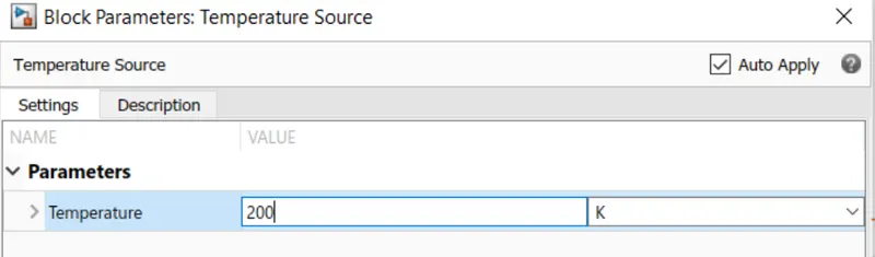
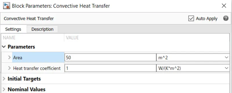
And the area in the convective heat transfer was made to 50m^2, and th coefficient to 1 also here we made the temperature 200k

Let's see the result

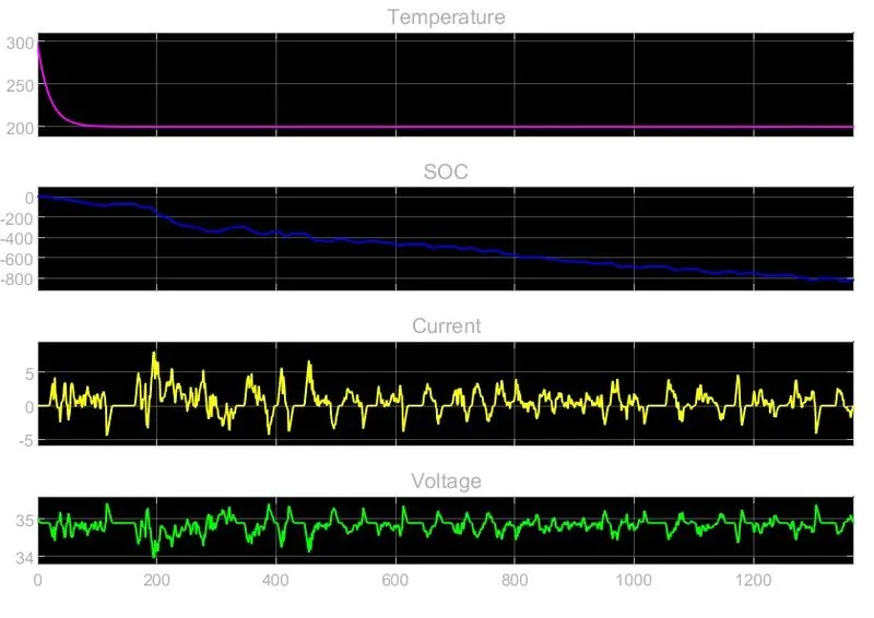
Due to no modifications being made on the load side, the current is the same as it was above.
Since the running duration is so tiny, we cannot see any differences in the second graph, which is a SOC, as I previously said.
The first graph, which shows temperature as a function of time, has been altered similarly to the first and second ones. It begins at 300 and drops until 200, at which point it becomes constant.
So, certainly, we have noticed the stark contrast between this one and the previous one.

Conclusion:-

The cycle of charge and discharge is not very variable here due to temperature differences, but in real life, it must be variable because the temperature of the battery fluctuates by varying the outside temperature supplied.