Project 2 - Speed Control of a Direct Current (DC) motor

Answer -

The DC motor has a mechanical part and an electrical part that needs to be modelled. The electrical energy is converted to form a mechanical energy in the form of rotation of mechanical parts. The change in supply voltage gives rise to magnetic field around rotor that gets repelled by the stator due to interacting magnetic field. The circuit contains two circuits - 1) Armature circuit and 2) Field circuit.

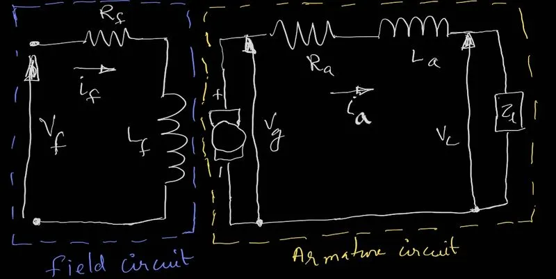
The circuit circled in purple in the above image is field circuit containing elements field resistance (`R_f`), field inductance (`L_f`), field current (`i_f`) and field voltage (`V_f`). The circuit encircled in yellow dscribes the armature circuit which contains elements armature resistance (`R_a`), armature inductance (`L_a`), load, armature current (`i_a`), load voltage (`V_L`) and generated voltage (`V_g`). The circular element in the armature is the rotating element of the machine that produces mechanical energy.

The objective of the challenge is to model the armature ciruit in simulink and implement PID control gains to understand the settling time, overshoot and steady state error percent.

Applying Newton's second law to the armature circuit gives -

`J * ddottheta + B * dottheta = K_T * i_a` `

Applying Kirchhoff's closed loop law to the armature circuit gives -

`L_a* doti_a + R_a * i_a = V - K_b * dottheta`

Converting the above to transfer functions -

`(theta(s)) / (V(s)) = K_T / (s*(L_a * s + R_a)* (J*s + B) + K_T*K_b`

`(omega(s))/(V(s)) = K_T / ((L_a*s + R_a) * (J*s + B) + K_T*K_b)`

The PD gain parameters are estimated by pole mapping method and the Integral gain is optimised in an iterative method. The poles are estimated by the following equation

`P = -zeta*omega_n pm omega_n * (sqrt(zeta^2 - 1) )`

The place command is further used to calculate the gains with the above mentioned poles.

The overshoot and steady state error percentage are estimated by the below formulae -

Overshoot (in %) = `100 * e^ (-((zeta * pi)/ (sqrt(1 - zeta^2))))`

Percent error = `(Estimated Value - Actual Value)/ (Actual Value) * 100`

The below is the code of the M-script

clear all;
close all;
clc;

%% Initializing the parameters
J = 0.01; % kgm^2 - Moment of inertia of the rotor
Bm = 0.1; % Nms - Motor viscous friction constant
Km = 0.01; % V/(rad/s) - Back EMF constant
Kt = 0.01; % Nm/A - Motor torque constant
Ra = 1; % ohm - Armature resistance
La = 0.5; % Henry - Armature inductance

%% Iitializing parameters for the PID
A = [-Bm/J, Kt/J; -Km/La, -Ra/La]; 
B = [0; 1/La];
zeta = 0.5;
fn = 1; % Natural frequency in Hz
wn = 2*pi*fn; 
p1 = -zeta*wn + wn*sqrt(zeta^2 - 1); % poles
p2 = -zeta*wn - wn*sqrt(zeta^2 - 1); % poles
p = [p1, p2];
K = place(A, B, p); % Proportional and Derivative gains
Ki = 20; % Integral gain

%% Running simulation 
data_PID = sim("DcMachine_ModelRun.slx");

%% Plotting the graphs
figure(1)
plot(data_PID.Time, data_PID.E_t, 'k--', data_PID.Time, data_PID.speed,'m-')
xlabel("Simulation Time")
ylabel("Speed")
legend('without PID', 'with PID')
title('Speed Regulation')
grid on

figure(2)
plot(data_PID.Time, data_PID.E_t, 'k--', data_PID.Time, data_PID.speed,'m-')
xlabel("Simulation Time")
ylabel("Speed")
legend('without PID', 'with PID')
title('Speed Regulation')
xlim([2, 5])
%ylim([64,66])
grid on

figure(3)
plot(data_PID.Time, data_PID.E_t, 'k--', data_PID.Time, data_PID.speed,'m-')
xlabel("Simulation Time")
ylabel("Speed")
legend('without PID', 'with PID')
title('Speed Regulation')
ylim([50, 160])
grid on

The simulink model images are as below -

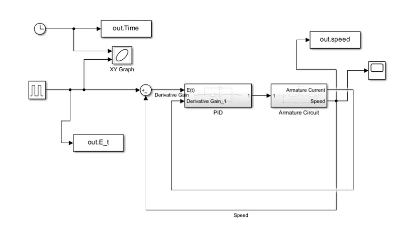
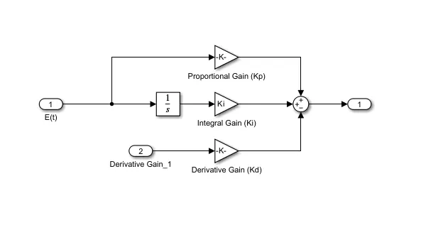
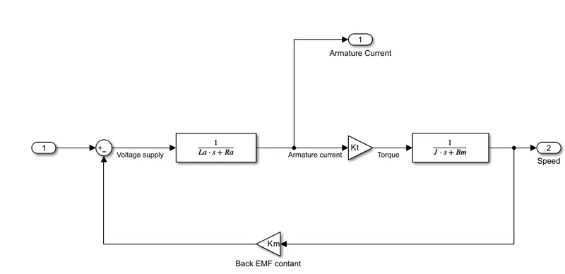
The sub-systems (a) PID controller and (b) Armature ciruit are expanded and their images as below -

(a) PID controller

(b) Armature circuit

RESULT -

The below are the plots that help determine the setting time, overshoot and steady state error percentage for an tuned values of the proportional, derivative and integral gain values.

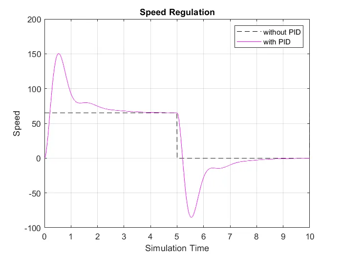
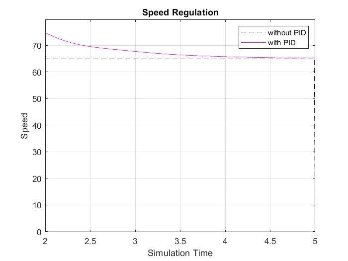
From the above image the settling time is approximately observed to be at 3 sec of the simulation time. The overshoot is calculated by the equation as mention above [equation number ] which is estimated to be 16.30% .

The image below is zoomed using axis limits which helps to determine the steady state error. The settling time approximated to be 3 secs, the value at that time is 67 of the magenta curve (with PID) and the actual value is 65 giving around 3 % of steady state error.