Project 1 - Data Handling and Interpolation

Project 1 -

The ode solvers in MATLAB are used to numerically solve ordinary differential equations. Out of which ode45 and ode23 are the most frequently used solvers that use the Runge-Kutta method to solve the equation which can help solve simple differential equations or simulate dynamic systems.

The ode23 differentiates the system equation using the second and third order Runge-Kutta method, showing moderate accuracy.

The ode45 differentiates the system equation using the four and fifth order Runge-Kutta approach, hence showing higher accuracy.

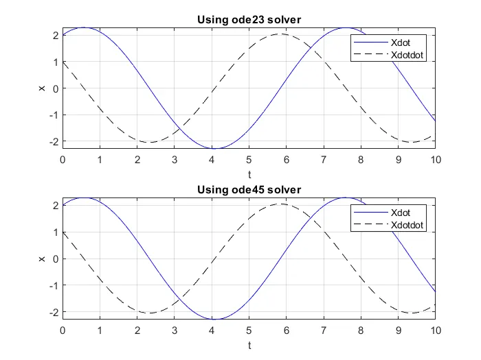
In this project a mass-spring system is modelled and solved using both the solvers for their thier position, velocity and acceleration to develop an understanding on the differences between the solvers.

The equation of the system is as follows -

`ddot X = -k/(mass) * X`

where mass = mass of the object

k = spring constant

The mass and the spring constant 'k' was to be defined by the user in the dialogue box that appears while excuting the code.

The above system can be represented in state space representation in the matrix form as below -

`[[dotx_2], [dotx_1]] = [[-k/(mass), 0], [0,1]] * [[x_1], [x_2]]`

The following is the main script for parameter initialization, function call, ode solvers and plotting command -

clear;
close all;
clc;

%% Intialising the parameters required to solve the equation.
prompt = ["m (in kg)", "k (in N/m)"];
param = inputdlg(prompt);
% Conversion of the parameters accepted in the dialoguebox from class cell format to class double
param = str2double(param);  
mass = param(1);
k = param(2);
t_span = 0:0.1:100;
x0 = [2; 1];

%% Computing the differential equations
[t, x] = ode23(@(t, x) simple_harmonic_motion(x, mass, k), t_span, x0); 

[t1, x1] = ode45(@(t1, x1) simple_harmonic_motion(x1, mass, k), t_span, x0);

%% Plotting figure
% subplot for the values using ode23
subplot(2,1,1)
plot(t, x(:,1), 'b-', t, x(:,2), 'k--')
xlabel("t")
ylabel("x")
title("Using ode23 solver")
legend(["Xdot","Xdotdot"])
xlim([0,10])
grid on

% subplot for the values using ode45
subplot(2,1,2)
plot(t1, x1(:,1), 'b-', t1, x1(:,2), 'k--')
xlabel("t")
ylabel("x")
title("Using ode45 solver")
legend(["Xdot","Xdotdot"])
xlim([0,10])
grid on

The following is the function script to evaluate the state vectors

function x_dot = simple_harmonic_motion(x, mass, k)

x_dot = zeros(2,1); % To create a matrix
x_dot(1) = x(2); % Equation dot_x = x(2)
x_dot(2) = - (k/mass) * x(1); % Equation dotdot_x = - k/mass * x

end

Result -

The below shows the velocity (x_dot) and acceleration (x_dotdot) using both solvers ode23 and ode45.

Project 2 -

The excel file provided in the question description is loaded in the MATLAB file which has data of elevation and temperature. The elevation data was split into three smaller parts that make it easy to fit the newer data of temperature.

The polyfit command is used to determine the coefficients of polynomial p(x) of degree n that is a best fit for the new temperature data.

Polyval command is then used to obtain the new temperature data by evaluating the polynomial p using the coffecients obtained at each point in x data that results in new temperature data.

Use the save command to save the new data into text file.

The code for the curvefit project is as below -

clear all;
close all;
clc;

%% Loading the table 
data = readmatrix("mini_project_2.xlsx");
elevation = data(:,1);
temperature = data(:,2);

E1 = elevation(1:27); T1 = temperature(1:27);
E2 = elevation(27:45); T2 = temperature(27:45);
E3 = elevation(45:50); T3 = temperature(45:50);

%% Computing the curvefit coefficients
[p1, S1] = polyfit(E1, T1, 1);
temp1 = polyval(p1, E1);

[p2, S2] = polyfit(E2, T2, 1);
temp2 = polyval(p2, E2);

[p3, S3] = polyfit(E3, T3, 1);
temp3 = polyval(p3, E3);

save('Temperature_NewData.txt',"temp1", "temp2", "temp3", "-ascii")

%% Plotting the data from table
figure(1)
plot(elevation, temperature, 'k-')
hold on 
plot(E1, temp1, 'B.')
hold on 
plot(E2, temp2, 'B.')
hold on 
plot(E3, temp3, 'B.')
xlabel("Elevation")
ylabel("Temperature")
title("Temperature vs Elevation")
legend(["Original curve", "Curvefit"])
grid on

Result -

The plot that shows the both old and new data is as below -

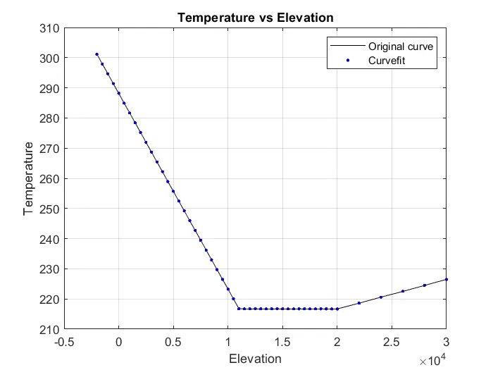
The black line represents the original data given in the excel sheet and the blue dots represents the new temperature data obtained by using the polyfit and polyval.

Comments on the goodness of fit. As seen in the plot the two curves are overlapping one another that shows using linear or polynomial of degree one is the best value to obtain a curve or data with high goodness of fit.

The text file is present in the zip folder attached to the answer.

Project 3 -

A function trigono_generator is made to evaluate the expression

`y = sin(x^2) + cos(x) - sin(2*x)`

And the objective of the project is to find local minima and global maxima of the above expression. The local minima being the point where the function is minimum at a specific interval and global maxima being a point where the function has the greatest value are some tools of optimization.

The following section contains the main script which is used -

clear;
close all;
clc;

%% Initializing input
x = 0:0.1:5;
%x0 = 0; 

%% Function call
y = trigono_generator(x);

%% Computing the local minima and global maxima
%options = optimset('PlotFcns', @optimplotfval);
[min_localx, min_localy] = fminsearch('trigono_generator(x)', 0);
[max_value, index_val] = max(y);

%% Plotting data
figure(1)
plot(x, y, 'k-') 
hold on
plot(min_localx, min_localy, 'ro', x(index_val), max_value, 'ro')
xlabel("x values")
ylabel("Trigonometric functions")
title("Trigonometric Expression")
gtext("Local minima")
gtext("Global maxima")
grid on

The following contains the code to the function that evaluates the y value for every x input

function y = trigono_generator(x)

%% Function that implements the below expression
y = sin(x.^2) + cos(x) - sin(2.*x);

end

Result -

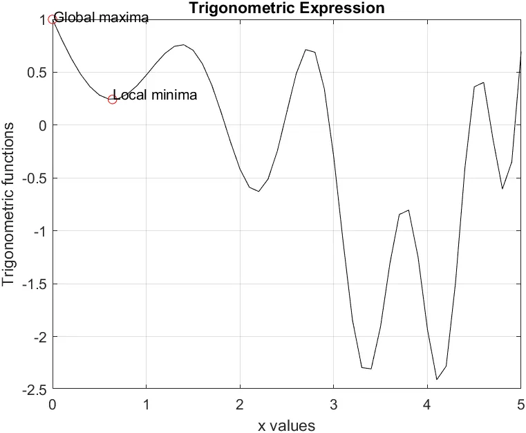
The local minima co-ordinates are (0.6392, 0.2423) and global maxima is obtained in the co-ordinates (0,1)

The following contains the plot with both local minima and global maxima

Project 4 -

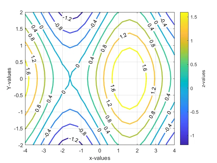
Contour plot helps to map the isolines of the z-matrix in x-y plane defining different magnitudes in different colour codes. The 'x' and 'y' matrices was generated in certain range (-4, 4) and (-2,2) respectively using meshgrid command. The z-value was evaluated by the following expression -

`Z = sin(x) + cos(Y)`

The matrix 'z' is then plotted as isoline with their magnitude mentioned in the plot. The following describes the code that helped to plot a contour plot -

clear all;
close all;
clc;

%% Initializing the values 
x = -4:0.4:4;
y = -2:0.2:2;
[X, Y] = meshgrid(x, y);

%% Computing expression 
z = sin(X) + cos(Y);                    

%% Plotting the contour plots
figure(1)
[c, h] = contour(X, Y, z, 'ShowText','on','LevelList',x);
w = h.LineWidth;
h.LineWidth = 2;
ylabel("Y-values")
xlabel("x-values")
grid on;
cb = colorbar;
cb.Location = 'eastoutside';
cb.Label.String = 'z-values';

Result -

The following shows the contour plot for the above example mentioned