Project 2 - Rankine cycle Simulator
The Rankine cycle, also referred as the Rankine Vapor Cycle, is a process that is frequently employed by power plants such as coal-fired power plants and nuclear reactors. A fuel is used to generate heat within a boiler, transforming water into steam, which then expands through a turbine, providing usable work. Scottish engineer William J.M. Rankine invented this technique in 1859. This thermodynamic cycle turns heat into mechanical energy, which is then turned into electricity by electrical generation.
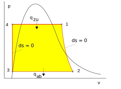
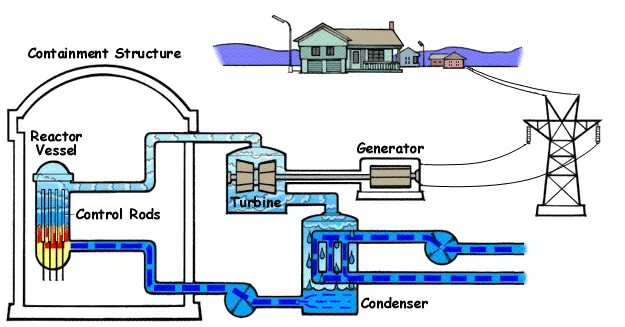
The steps in the Rankine Cycle as shown in Figure 1 and the corresponding steps in the pressure-volume (figure 2) are outlined below:
- Pump: Compression of the fluid to high pressure using a pump (this takes work) (Figure 2: Steps 3 to 4)
- Boiler: The compressed fluid is heated to the final temperature (which is at boiling point), therefore, a phase change occurs—from liquid to vapor. (Figure 2: Steps 4 to 1)
- Turbine: Expansion of the vapor in the turbine. (Figure 2: Steps 1 to 2)
- Condenser: Condensation of the vapor in the condenser (where the waste heat goes to the final heat sink (the atmosphere or a large body of water (ex. lake or river). (Figure 2: Steps 2 to 3)
The efficiency of the Rankine cycle is limited by the high heat of vaporization by the fluid. The fluid must be cycled through and reused constantly, therefore, water is the most practical fluid for this cycle. This is not why many power plants are located near a body of water—that's for the waste heat.
As the water condenses in the condenser, waste is given off in the form of water vapour—which can be seen billowing from a plant's cooling towers. This waste heat is necessary for any thermodynamic cycle. Due to this condensation step, the pressure at the turbine outlet is lowered. This means the pump requires less work to compress the water—resulting in higher overall efficiencies.
Processes in the Rankine cycle - There are four processes in the Rankine cycle.
- Process 1–2: The dry saturated vapor expands through a turbine, generating power. This decreases the temperature and pressure of the vapor, and some condensation may occur. The output in this process can be easily calculated using the chart or tables noted above. Process 1-2 is isentropic expansion.
- Process 2–3: The wet vapor then enters a condenser, where it is condensed at a constant pressure to become a saturated liquid. Process 2-3 is constant pressure heat rejection in the condenser.
- Process 3–4: The working fluid is pumped from low to high pressure. As the fluid is a liquid at this stage, the pump requires little input energy. Process 3-4 is isentropic compression.
- Process 4–1: The high-pressure liquid enters a boiler, where it is heated at constant pressure by an external heat source to become a dry saturated vapor. The input energy required can be easily calculated graphically, using an enthalpy–entropy chart (h–s chart), or numerically, using steam tables or software. Process 4-1 is constant pressure heat addition in the boiler.
In an ideal Rankine cycle, the pump and turbine would be isentropic, i.e., the pump and turbine would generate no entropy and hence maximize the network output. Processes 1–2 and 3–4 would be represented by vertical lines on the T–s diagram and more closely resemble that of the Carnot cycle. The Rankine cycle shown here prevents the state of the working fluid from ending up in the superheated vapor region after the expansion in the turbine, which reduces the energy removed by the condensers.
------------------------------------------------------------------------------------------------------------------
MAIN CODE
clear all
close all
clc
disp(' RANKINE CYCLE ');
disp('1-2 is Constant pressure heat addition in the boiler');
disp('2-3 is Isentropic Expansion in the Turbine');
disp('3-4 is Constant pressure heat removal in the Condenser');
disp('4-1 is Isentropic compression in the pump');
p1 = input('nValue of pressure at turbine inlet, p1(in bar) = ');
T1 = input('nValue of temperature at turbine inlet, T1(in degree.C) = ');
p2 = input('nValue of pressure at condenser inlet, p2(in bar) = ');

% Properties at state 1
h1=XSteam('h_pT',p1,T1)
s1=XSteam('s_pT',p1,T1)

% Properties at state 2
s2 = s1;                            % Isentropic Expansion
sf2= XSteam('sL_p', p2);            % Saturated Liquid Entropy
sg2 = XSteam('sV_p', p2);           % Saturated Vapour Entropy
x2 = (s2-sf2)/(sg2-sf2);
hf2 = XSteam('hL_p', p2);
hg2 = XSteam('hV_p', p2);
h2 = hf2 + (x2*(hg2-hf2));

% At State 3
p3 = p2;                            % Constant pressure Heat rejection in Condenser
s3= XSteam('sL_p', p3);
h3 = XSteam('hL_p', p3);

% At State 4
s4 = s3;
p4 = p1;

% Calculation of Temperatures at the state points
T3 = XSteam('Tsat_p', p3);
T2 = T3;
Cp4 = XSteam('Cp_ps', p4, s4);
Cv4 = XSteam('Cv_ps', p4, s4);
k = Cp4/Cv4;
T4 = T3/((p3/p4)^((k-1)/k));

% At State 4
s4 = s3;
p4 = p1;

% Work done by turbine
Wt = h1 - h2;

% Work done to run pump
v3 = XSteam('vL_p', p3);
Wp = v3*(p4 - p3)*100;
h4 = h3 + Wp;

%Net work
Wnet = Wt - Wp;

%Heat into the system
Qin = h1 - h4;

%Heat out of the system
Qout = h2 - h3;

%Thermal efficiency
thermal_eff = (Wnet/Qin)*100;

%Specific Steam Consumption
%SSC = mass flow rate/power
SSC = (3600/Wnet);

% Back Work ratio
BW = (Wp/Wt)


% Calculation of Temperatures at the state points
T3 = XSteam('Tsat_p', p3);
T2 = T3;
Cp4 = XSteam('Cp_ps', p4, s4);
Cv4 = XSteam('Cv_ps', p4, s4);
k = Cp4/Cv4;
T4 = T3/((p3/p4)^((k-1)/k));

%Calculating Temperature, Entropy and Enthalpy at the vapour and liquid line for plotting
T6 = XSteam('Tsat_p', p1);
s5 = XSteam('sL_p', p1);
s6 = XSteam('sV_p', p1);
h5 = XSteam('hL_p', p1);
h6 = XSteam('hV_p', p1);
T5 = T6;


%Plotting the saturation curve
T = linspace(1,375,1000);
for i = 1:length(T)

sf(i) = XSteam('sL_T', T(i));
sg(i) = XSteam('sV_T', T(i));
hf(i) = XSteam('hL_T', T(i));
hg(i) = XSteam('hV_T', T(i));
end

%Plotting T-s diagram
figure(1)
hold on
plot(sf, T, 'r','linewidth',1)
plot(sg, T, 'r','linewidth',1)
plot([s1 s2], [T1 T2], 'b', 'linewidth', 2)
plot([s2 s3], [T2 T3] ,'b', 'linewidth', 2)
plot([s3 s4], [T3 T4], 'b', 'linewidth', 2)
plot([s4 s5], [T4 T5], 'b', 'linewidth', 2)
plot([s5 s6], [T5 T6], 'b', 'linewidth', 2)
sc1 = linspace(s6, s1, 1000);
for l = 1:length(sc1)
 Tc1(l) = XSteam('T_ps', p1, sc1(l));
end
plot(sc1, Tc1, 'b', 'linewidth', 2)
text(s1+0.1, T1, '1')
text(s2+0.1, T2, '2')
text(s3, T3-20, '3')
text(s4, T4+20, '4')
title('Temp vs Entropy plot')
xlabel('Entropy ,S (Kj/kgk')
ylabel('Temperature (degree C) ')
legend('Saturation curve')


%Plotting h-s diagram
figure(2)
hold on
plot(sf, hf, 'k', 'linewidth', 1)
plot(sg, hg, 'k',  'linewidth', 1)
plot([s1 s2], [h1 h2], 'r', 'linewidth', 2)
plot([s2 s3], [h2 h3], 'r', 'linewidth', 2)
plot([s3 s4], [h3 h4], 'r', 'linewidth', 2)
hc = linspace(h4, h5, 100);
for r = 1:length(hc)
sch(r) = XSteam('s_ph', p1, hc(r));
end
plot(sch,hc, 'r', 'linewidth', 2)
plot([s5 s6], [h5 h6], 'r', 'linewidth', 2)
for m = 1:length(sc1)
hc1(m) = XSteam('h_ps', p1, sc1(m));
end
plot(sc1, hc1, 'r', 'linewidth', 2)
text(s1+0.1, h1, '1')
text(s2+0.1, h2, '2')
text(s3, h3-100, '3')
text(s4, h4 +200, '4')
title('Enthalpy vs Entropy plot')
xlabel('Entropy , S (KJ/kgk) ')
ylabel('Enthalpy , H (KJ/kg)')
legend('Saturation curve','location','northwest')


% Displaying the Results in the Command Window:
disp('Results');
p1 = p1;
T1 = T1;
p2 = p2;
disp('At stage point 1');
n1 = sprintf('P1 is %.3f bar',p1);
disp(n1);
n2 = sprintf('T1 is %.3f C',T1);
disp(n2);
n3 = sprintf('h1 is %.3f kJ/kg',h1);
disp(n3);
n4 = sprintf('s1 is %.3f kJ/kgK',s1);
disp(n4);
disp('At stage point 2');
n11 = sprintf('P2 is %.3f bar',p2);
disp(n11);
n21 = sprintf('T2 is %.3f C',T2);
disp(n21);
n31 = sprintf('h2 is %.3f kJ/kg',h2);
disp(n31);
n41 = sprintf('s2 is %.3f kJ/kgK',s2);
disp(n41);
disp('At stage point 3');
n12 = sprintf('P3 is %.3f bar',p3);
disp(n12);
n22 = sprintf('T3 is %.3f C',T3);
disp(n22);
n32 = sprintf('h3 is %.3f kJ/kg',h3);
disp(n32);
n42 = sprintf('s3 is %.3f kJ/kgK',s3);
disp(n42);
disp('At stage point 4');
n13 = sprintf('P4 is %.3f bar',p4);
disp(n13);
n23 = sprintf('T4 is %.3f C',T4);
disp(n23);
n33 = sprintf('h4 is %.3f kJ/kg',h4);
disp(n33);
n43 = sprintf('s4 is %.3f kJ/kgK',s4);
disp(n43);
n14 = sprintf('Wt is %.3f kJ/kg',Wt);
disp(n14);
n15 = sprintf('Wp is %.3f kJ/kg',Wp);
disp(n15);
n16 = sprintf('Wnet is %.3f kJ/kg',Wnet);
disp(n16);
n17 = sprintf('Thermal_efficiency is %.2f Percent',thermal_eff);
disp(n17);
n18 = sprintf('SSC is %.2f kg/kWh',SSC);
disp(n18);
n19 = sprintf('Back work ratio is %.3f ',BW);
disp(n19);
Description of the Program
- Xsteam data is used to extract steam and water parameters such as enthalpy and entropy at specific temperature and pressure values for saturated liquid and saturated vapor situations, among others.
- The software requires an input of pressure (in bar) at state point 1 (turbine inlet), temperature (degree Celsius) at the same point, and pressure at the condenser inlet (point 2).
- The program calculates all of the Rankine cycle's state points using these inputs and Xsteam data.
- h1 = XSteam('h pT', p1, T1) provides the enthalpy of water at given pressure and temperature in bar and degrees Celsius, respectively.
- When the data is extracted, thermodynamic relationships were employed to locate more state points and extract their data from XSteam, as described after researching the Rankine cycle.
- Sf and sg, hf and hg, where f and g represent saturated liquid and saturated vapor, respectively, are calculated after examining Rankine cycle graphs and extracting data from an Xsteam file.
- The net work output, turbine work, pump work, heat in and heat out were all calculated using conventional thermodynamic relationships.
- The Rankine cycle's efficiency and specific steam consumption (s.s.c.) are determined using thermodynamic relations and mentioned in the program using relations.
- T, s, and h are retrieved at the vapor and liquid lines for plotting purposes, after the fourth point for the variance that can be observed in the figure.
- In T-S, the saturation curve is shown in red for saturated liquid and saturated gas, while in H-S, it is shown in black.
- Plot of T versus s and h vs s is generated from all the points collected from the program using the plot command and mentioning all the labels, linewidth, colour, and title.
-
For the above-mentioned inputs, the plot varies as the user input changes. The 'sprint' command displays the results in the command window.
- For every process phases of the water i.e liquid and vapor/gas are also considered. At state points 4 and 1 saturation process takes place where water is boiled and converted into a saturated liquid state and then it is converted to the saturated vapor state and then due to more boiling inside the boiler is converted to a superheated state. Two different phases are taking place between state points 4 and 1 hence temperature, enthalpy, and entropy for both the phases are calculated.
- To create a saturation curve for T-s and h-s diagram different enthalpy and entropy values based on liquid state and vapor/gas state are being calculated using temperature as an array for values 0 to 400 considering 500 values in between them. Net work done is calculated by equating work done by the turbine and work done to run the pump, using the equation of Wnet. The back work ratio is calculated using the equation for Bwr.
- Plots are created for T-s and h-s using the ‘hold on’ command for all the state points. At first saturation, the curve is made for both the graphs using h and s values that were calculated with temperature array at different phases of water. Then all the state points are joined using the ‘plot’ command. The t-s and h-s diagram includes title, axis labels and legends, and ‘text’ command to show the state points of the graph.
Result:
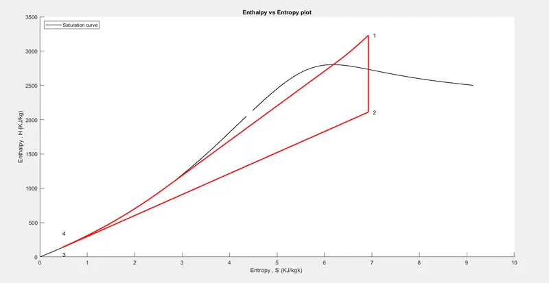
- Below are the T-s and h-s diagrams generated through the program based on the given inputs. Both diagrams represent the Rankine cycle and how temperature and enthalpy change in the complete cycle.
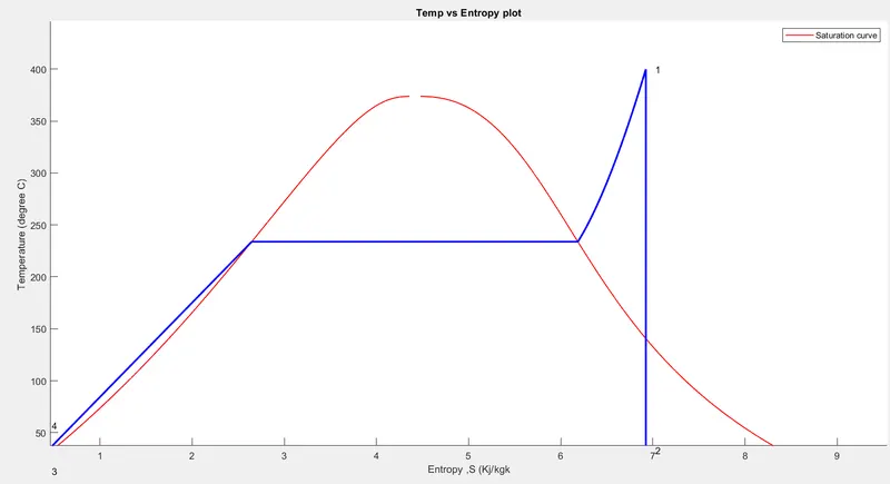
- In the T-s diagram, it can be seen how temperature changes throughout the process of the cycle. In the saturation curve, the left side is the saturated liquid state line and the right side is the saturated vapor/gas state line. In between state points [4-1] water changes from saturated liquid to saturated vapor/gas and then it goes to a superheated state. This is how high-pressure steam is formed.
RANKINE CYCLE
1-2 is Constant pressure heat addition in the boiler
2-3 is Isentropic Expansion in the Turbine
3-4 is Constant pressure heat removal in the Condenser
4-1 is Isentropic compression in the pump
nValue of pressure at turbine inlet, p1(in bar) = 30
nValue of temperature at turbine inlet, T1(in degree.C) = 400
nValue of pressure at condenser inlet, p2(in bar) = 0.05

h1 =

   3.2316e+03


s1 =

    6.9233


BW =

    0.0027

Results
At stage point 1
P1 is 30.000 bar
T1 is 400.000 C
h1 is 3231.571 kJ/kg
s1 is 6.923 kJ/kgK
At stage point 2
P2 is 0.050 bar
T2 is 32.875 C
h2 is 2110.708 kJ/kg
s2 is 6.923 kJ/kgK
At stage point 3
P3 is 0.050 bar
T3 is 32.875 C
h3 is 137.765 kJ/kg
s3 is 0.476 kJ/kgK
At stage point 4
P4 is 30.000 bar
T4 is 36.935 C
h4 is 140.776 kJ/kg
s4 is 0.476 kJ/kgK
Wt is 1120.863 kJ/kg
Wp is 3.011 kJ/kg
Wnet is 1117.852 kJ/kg
Thermal_efficiency is 36.17 Percent
SSC is 3.22 kg/kWh
Back work ratio is 0.003
Above are the values of all the state variables, the Net work done, the Back work ratio, and all rest of the variables to calculate the same.
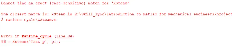
ERROR
1.
2.
