Project 2 - Rankine cycle Simulator

Aim:

1)Create a Rankine Cycle Simulator using MATLAB

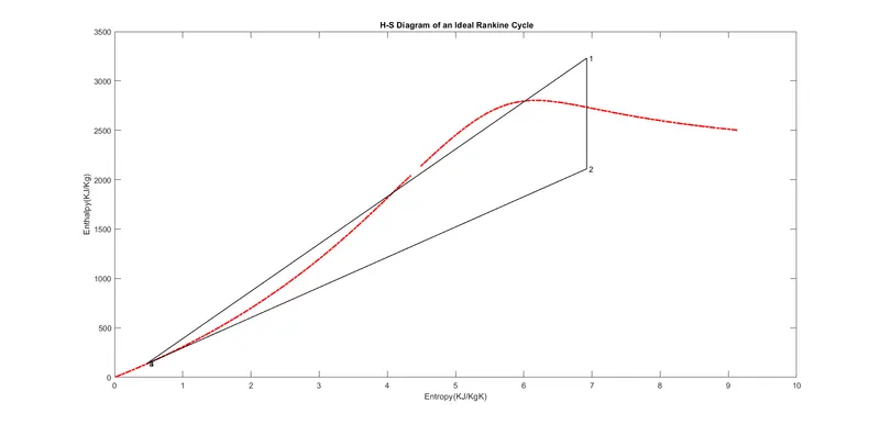
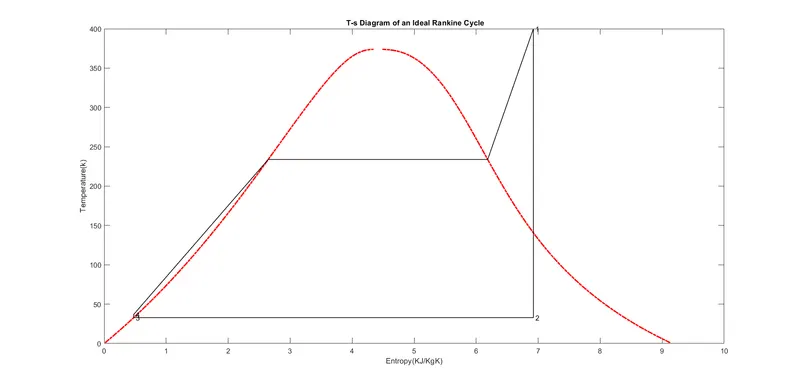
2)plot H-S diagram,T-S diagram for Rankine cycle

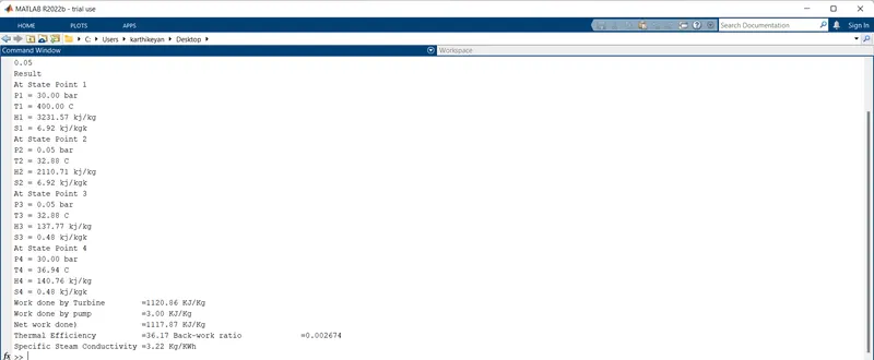
3)Display the state points of rankine cycle

4)calculate:Thermal efficiency,Back work ratio,Net wrok output

Inputs:

Turbine Inlet temperature = 400° C=t1

Turbine Inlet Pressure = 30 bars=p1

Turbine Outlet Pressure = 0.05 bars = Condenser Inlet Pressure=p2

Theory of Rankine cycle:

Thermodynamic cycles:

Thermodynamic cycles can be divided into two general categories: power cycles, which produce a net power output, and refrigeration and heat pump cycles, which consume a net power input. The thermodynamic power cycles can be categorized as gas cycles and vapor cycles. In gas cycles, the working fluid remains in the gas phase throughout the entire cycle. In vapor cycles, the working fluid exits as vapor phase during one part of the cycle and as liquid phase during another part of the cycle.Steam power plants run vapor power cycles with water as the working fluid. This section introduces the ideal cycle for vapor power cycle - Rankine cycle.

Rankine cycle - the Ideal Cycle for Vapor Power Cycle:

Vapor power plants generate electrical power by using fuels like coal, oil or natural gas. The schematic of a vapor power plant is shown on the left. The entire power plant can be broken down into four major subsystems.

• Subsystem A: Energy conversion from heat to work
• Subsystem B: Energy source and waste removal required to vaporize the water
• Subsystem C: Electric generator
• Subsystem D: Cooling water system

schematic of a Vapor Power Plant

The thermodynamic cycle in subsystem A is called the Rankine cycle. Subsystem A consists of a boiler, turbine, condenser and a pump. Fuel, burned in the boiler, heats the water to generate superheated steam (subsystem B). This steam is used to run the turbine which powers the generator. Electrical energy is generated when the generator windings rotate in a strong magnetic field (subsystem C). After the steam leaves the turbine, it is cooled to its liquid state in the condenser by transferring heat to the cooling water system (subsystem D). The liquid is pressurized by the pump prior to going back to the boiler.

All four components associated with the ideal Rankine cycle are steady-flow devices, and thus all four processes that make up the Rankine cycle can be analyzed as steady-flow process. The kinetic and potential energy changes of water are small relative to the heat and work terms, are thus neglected. Energy analysis of the four components are given below.

Pump (process 1-2): Pump pressurized the liquid water from the condenser prior to going back to the boiler. Assuming no heat transfer with the surroundings,

the energy balance in the pump is

w_{pump, in} = h₂ - h₁

_{Boiler (process 2-3): Liquid water enters the boiler and is heated to superheated state in the boiler.}

_{The energy balancein the boiler is}

_{Qin = h3 - h2}

Turbine (process 3-4): Steam from the boiler, which has an elevated temperature and pressure, expands through the turbine to produce work and then is discharged to the condenser with relatively low pressure. Neglecting heat transfer with the surroundings, the energy balance in the turbine is

w_{turbine, out} = h₃ - h₄

Condenser (process 4-1): Steam from the turbine is condensed to liquid water in the condenser. The energy balance in the condenser is

q_out = h₄ - h₁

For the whole cycle, the energy balance can be obtained by summarizing the four energy equations above. It yields,

(q_in- q_out) - (w_{turbine, out} - w_{pump, in}) = 0

The thermal efficiency of the Rankine cycle is determined from

η_th = w_{net ,out}/q_in = 1 - q_out/q_in

where the net work output from the cycle is

w_{net ,out} = w_{turbine, out} - w_{pump, in}

The Rankine cycle is an ideal cycle if water passes through the four components without irreversibilities and pressure drops. The ideal Rankine cycle consists of the following four processes, as shown on the T-s diagram on the left:

• 1-2: Isentropic compression in a pump
• 2-3: Constant pressure heat addition in a boiler
• 3-4: Isentropic expansion in a turbine
• 4-1: Constant pressure heat rejection in a condenser

T-s Diagram of an Ideal Rankine Cycle

Program code:

%Program to Simulate Rankine Cycle
clear all
close all
clc

% User Inputs
p1 = input('Enter the Pressure at the Turbine Inlet (in bar):\n');
t1 = input('Enter the Temperature at the Turbine Inlet (in Degree Celcius):\n');
p2 = input('Enter the Pressure at the Condenser Inlet (in bar):\n');

%Turbine Inlet
s1 = XSteam('s_pT',p1,t1);
h1 = XSteam('h_pT',p1,t1);

%Condenser Inlet
s2 = s1;
sf2=XSteam('sL_p',p2);
sg2=XSteam('sV_p',p2);
hf2=XSteam('hL_p',p2);
hg2=XSteam('hV_p',p2);
%`Determining Dryness fraction`
if(s2 <= sg2)
    x2 = ((s2 - sf2) / (sg2 - sf2));
else
    x2 = 1;    
end
h2 = hf2 + (x2 * (hg2 - hf2));

%Pump Inlet
p3 = p2;
t3 = XSteam('Tsat_p',p3);
s3 = XSteam('sL_p',p3);
h3 = XSteam('hL_p',p3);
t2 = t3;

%Boiler Inlet 
p4 = p1; 
s4 = s3; 
h4 = XSteam('h_ps',p4,s4);
cp = XSteam('Cp_ps',p4,s4);   %Isobaric specific heat
cv = XSteam('Cv_ps',p4,s4);   %Isochoric specific heat
%Determining Gamma
gamma = ( cp / cv );
t4 = (t3 * (( p3 / p4 )^(( 1 - gamma) / gamma)));

%Work Done
%Work Done by the Turbine
Wt = h1 - h2;
%Work Done by the Pump
Wp = h4 - h3;
%Net Work Done
Wnet = Wt - Wp;

%Heat Added
%Heat Added in the Boiler
qin = h1 - h4;
%Heat Rejected in the Condensor
qout = h2 - h3;

%Thermal Efficiency
n = (Wnet / qin) * 100;

%Specific Steam Consumption
SSC = (3600/Wnet);

%Back work ration
bwr=Wp/Wt;


%Result
fprintf('Result \n');
fprintf('At State Point 1 \n');
fprintf('P1 = %.2f bar \n',p1)
fprintf('T1 = %.2f C \n',t1)
fprintf('H1 = %.2f kj/kg \n',h1)
fprintf('S1 = %.2f kj/kgk \n',s1)

fprintf('At State Point 2 \n');
fprintf('P2 = %.2f bar \n',p2)
fprintf('T2 = %.2f C \n',t2)
fprintf('H2 = %.2f kj/kg \n',h2)
fprintf('S2 = %.2f kj/kgk \n',s2)

fprintf('At State Point 3 \n');
fprintf('P3 = %.2f bar \n',p3)
fprintf('T3 = %.2f C \n',t3)
fprintf('H3 = %.2f kj/kg \n',h3)
fprintf('S3 = %.2f kj/kgk \n',s3)

fprintf('At State Point 4 \n');
fprintf('P4 = %.2f bar \n',p4)
fprintf('T4 = %.2f C \n',t4)
fprintf('H4 = %.2f kj/kg \n',h4)
fprintf('S4 = %.2f kj/kgk \n',s4)

fprintf('Work done by Turbine        =%.2f KJ/Kg \n',Wt)
fprintf('Work done by pump           =%.2f KJ/Kg \n',Wp)
fprintf('Net work done)              =%.2f KJ/Kg \n',Wnet)
fprintf('Thermal Efficiency          =%.2f % \n',n)
fprintf('Back-work ratio             =%f  \n',bwr)
fprintf('Specific Steam Conductivity =%.2f Kg/KWh \n',SSC)


%Plotting
%TS Diagram
t = linspace(1,t1,2000);
for i = 1: 2000
    sl(i) = XSteam('sL_T',t(i));
end
for i = 1: 2000
    sv(i) = XSteam('sV_T',t(i));
end
figure(1)
plot(sl,t,'-.r','LineWidth',2)
hold on
plot(sv,t,'-.r','LineWidth',2)
title(' T-s Diagram of an Ideal Rankine Cycle')
xlabel('Entropy(KJ/KgK)')
ylabel('Temperature(k)')
%1-2 State
plot([s1 s2],[t1 t2],'k','LineWidth',1)
%2-3 State
plot([s2 s3],[t2 t3],'k','LineWidth',1)
%3-4 State
plot([s3 s4],[t3 t4],'k','LineWidth',1)
%4-1 State
tp = XSteam('TSat_p',p4);
sp = XSteam('sL_T',tp);
tq = tp;
sq = XSteam('sV_T',tq);
plot([s4,sp],[t4,tp],'k','LineWidth',1)
plot([sp sq],[tp tq],'k','LineWidth',1)
plot([sq,s1],[tq,t1],'k','LineWidth',1)
text(s1,t1,' 1');
text(s2,t2,' 2');
text(s3,t3,' 3');
text(s4,t4,' 4');

%PV Diagram
for i = 1: 2000
    hl(i) = XSteam('hL_T',t(i));
end
for i = 1: 2000
    hv(i) = XSteam('hV_T',t(i));
end
figure(2)
plot(sl,hl,'-.r','LineWidth',2)
hold on
plot(sv,hv,'-.r','LineWidth',2)
title(' H-S Diagram of an Ideal Rankine Cycle')
xlabel('Entropy(KJ/KgK)')
ylabel('Enthalpy(KJ/Kg)')
%1-2 State
plot([s1 s2],[h1 h2],'k','LineWidth',1)
%2-3 State
plot([s2 s3],[h2 h3],'k','LineWidth',1)
%3-4 State
plot([s3 s4],[h3 h4],'k','LineWidth',1)
%4-1 State
plot([s4 s1],[h4 h1],'k','LineWidth',1)
text(s1,h1,' 1');
text(s2,h2,' 2');
text(s3,h3,' 3');
text(s4,h4,' 4');

Output results:

Output plots:

TS plot:

HS plot: