Project 2 - Rankine cycle Simulator

Aim

To create a Rankine cycle simulator and plot the corresponding T-S and H-S plots using MATLAB.

Objective

• Create a Rankine Cycle Simulator using MATLAB.
• Plot the corresponding T-s and h-s plots for the given set of inputs.
• Make a report explaining the working of a rankine cycle simulator.
• Calculate Net work output and back work ratio.

Rankine Cycle

The Rankine cycle is an idealized thermodynamic cycle describing the process by which certain heat engines such as steam turbines or reciprocating steam engines, allow mechanical work to be extracted from a fluid as it moves between a heat source and heat sink. Heat energy is supplied to the system via a boiler where the working fluid (typically water) is converted to a high pressure gaseous state (steam) in order to turn a turbine. After passing over the turbine the fluid is allowed to condense back into a liquid state as waste heat energy is rejected before being returned to boiler, completing the cycle. Rankine engines generally operate in a closed loop where the working fluid is reused. While many substances can be used as the working fluid, water is usually chosen for its simple chemistry, relative abundance, low cost, and thermodynamic properties. y condensing the working steam vapor to a liquid the pressure at the turbine outlet is lowered and the energy required by the feed pump consumes only 1% to 3% of the turbine output power and these factors contribute to a higher efficiency for the cycle. The ability of a Rankine engine to harness energy depends on the relative temperature difference between the heat source and heat sink. The greater the differential, the more mechanical power can be efficiently extracted out of heat energy, as per Carnot's theorem.

There are four processes in the Rankine cycle. The states are identified by numbers in the T-S Diagram:

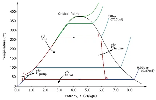
• Process 1–2: The working fluid is pumped from low to high pressure. As the fluid is a liquid at this stage, the pump requires little input energy. Process 1-2 is isentropic compression.
• Process 2–3: The high-pressure liquid enters a boiler, where it is heated at constant pressure by an external heat source to become a dry saturated vapour. Process 2-3 is constant pressure heat addition in boiler.
• Process 3–4: The dry saturated vapour expands through a turbine, generating power. This decreases the temperature and pressure of the vapour, and some condensation may occur. Process 3-4 is isentropic expansion.
• Process 4–1: The wet vapour then enters a condenser, where it is condensed at a constant pressure to become a saturated liquid. Process 4-1 is constant pressure heat rejection in condenser.

Governing Equations

Work done on pump, per kg of water:

Wp = v3(p4-p3)*100

Heat energy added in steam generator:

Qin = h3-h2

Work done by turbine:

Wt = h1-h2

Heat energy rejected in the condenser:

Qout = h4-h1

Net-Work done is given by:

Wnet = Wt - Wp

The thermal efficiency of the Rankine cycle is given by:

nth = (Wnet/Qin)*100

Back Work Ratio is given by:

BWR = Wp/Wt where,

h = Enthalpy (1,2,3,4 are different state points)

v = volume

p = pressure

Codes

The code or program to create a Rankine cycle simulator and plot the corresponding T-S and H-S plots using MATLAB is given below:

% Rankine Cycle Simulator

clear all
close all
clc

% Printing Introduction
fprintf('Rankine cycle simulator \n')
fprintf('1-2 is isentropic expansion in turbine \n')
fprintf('2-3 is constant pressure heat rejection by the condenser \n')
fprintf('3-4 is isentropic compression in pump \n')
fprintf('4-1 is constant pressure heat addition by the boiler \n')

% User inputs
p1 = input(' Enter the pressure at the turbine inlet (in bar): ');
t1 = input(' Enter the temperature at the turbine inlet (in Degree celcius): ');
p2 = input(' Enter the pressure at the turbine outlet (in bar): ');

% State point 1
h1 = XSteam('h_pt',p1,t1);           % Enthalpy
s1 = XSteam('s_pt',p1,t1);           % Entropy
hf1 = XSteam('hL_p',p1);             % Enthalpy of saturated liquid
hg1 = XSteam('hV_p',p1);             % Enthalpy of saturated vapour
sf1 = XSteam('sL_p',p1);             % Entropy of saturated liquid
sg1 = XSteam('sV_p',p1);             % Entropy of saturated vapour
ts1 = XSteam('Tsat_p',p1);           % Saturation temperature
fprintf('At state point 1\n')
fprintf('p1 is : %f bar\n',p1)
fprintf('t1 is : %f Deg celcius\n',t1)
fprintf('h1 is : %f KJ/Kg\n',h1)
fprintf('s1 is : %f KJ/Kg-K\n',s1)

% State point 2
s2 = s1;
hf2 = XSteam('hL_p',p2);
hg2 = XSteam('hV_p',p2);
sf2 = XSteam('sL_p',p2);
sg2 = XSteam('sV_p',p2);
x = (s2-sf2)/(sg2-sf2);              % Dryness fraction
h2 = hf2 + x*(hg2-hf2);
t2 = XSteam('T_ph',p2,h2);
ts2 = XSteam('Tsat_p',p2);
fprintf('At state point 2\n')
fprintf('p2 is : %f bar\n',p2)
fprintf('t2 is : %f Deg celcius\n',t2)
fprintf('h2 is : %f KJ/Kg\n',h2)
fprintf('s2 is : %f KJ/Kg-K\n',s2)

% State point 3
h3 = hf2;
s3 = sf2;
t3 = t2;
p3 = p2;
v3 = XSteam('vL_p',p3);
fprintf('At state point 3\n')
fprintf('p3 is : %f bar\n',p3)
fprintf('t3 is : %f Deg celcius\n',t3)
fprintf('h3 is : %f KJ/Kg\n',h3)
fprintf('s3 is : %f KJ/Kg-K\n',s3)

% State point 4
p4 = p1;
s4 = s3;
Wp = v3*(p4-p3)*100;                      % Wp = work done by pump
h4 = Wp + h3;
t4 = XSteam('T_ps',p4,s4);
fprintf('At state point 4\n')
fprintf('p4 is : %f bar\n',p4)
fprintf('t4 is : %f Deg celcius\n',t4)
fprintf('h4 is : %f KJ/Kg\n',h4)
fprintf('s4 is : %f KJ/Kg-K\n',s4)

% Temperature space for saturation curve and cycle
t = linspace(0,373,500);
for i = 1:length(t)
    h_l(i) = XSteam('hL_t',t(i));    % Enthalpy of liquid
    h_v(i) = XSteam('hV_t',t(i));    % Enthalpy of vapour
    s_l(i) = XSteam('sL_t',t(i));    % Entropy of liquid
    s_v(i) = XSteam('sV_t',t(i));    % Entropy of vapour
end

% Plot T-S Diagram
figure(1)
hold on
plot([s1 s2],[t1 t2],'LineWidth',2,'Color','r')
plot([s2 sg2],[t2 ts2],'LineWidth',2,'Color','r')
plot([sg2 s3],[ts2 t3],'LineWidth',2,'Color','r')
plot([s3 s4],[t3 t4],'LineWidth',2,'Color','r')
plot([s4 sf1],[t4 ts1],'LineWidth',2,'Color','r')
plot([sf1 sg1],[ts1 ts1],'LineWidth',2,'Color','r')
plot([sg1 s1],[ts1 t1],'LineWidth',2,'Color','r')
plot(s_l,t,'LineStyle','--','LineWidth',2,'Color','b')
plot(s_v,t,'LineStyle','--','LineWidth',2,'Color','b')
xlabel('Specific Entropy [KJ/KgK]')
ylabel('Temperature (degree celcius)')
title('T - S Diagram for Rankine Cycle')

% Plot H-S Diagram
figure(2)
hold on
plot([s1 s2 s3 s4 s1],[h1 h2 h3 h4 h1],'LineWidth',2,'Color','r')
plot(s_l,h_l,'LineStyle','--','LineWidth',2,'Color','b')
plot(s_v,h_v,'LineStyle','--','LineWidth',2,'Color','b')
xlabel('Specific Enthalpy [KJ/Kg]')
ylabel('Specific Entropy [KJ/KgK]')
title('H - S Diagram for Rankine Cycle')

% Calculation of Net work output and Back work ratio
% Work done by turbine
Wt = h1-h2;

% Heat addition
Qin = h1-h4;

% Net work output
Wnet = Wt - Wp;

% Thermal Efficiency
nth = (Wnet/Qin)*100;

% Back work ratio
BWR = Wp/Wt;

fprintf('Work done by turbine Wt is : %f kJ/kg\n', Wt)
fprintf('Work done by pump Wp is : %f kJ/kg\n', Wp)
fprintf('Thermal efficiency nth is : %f\n', nth)
fprintf('Net work output Wnet is : %f\n',Wnet)
fprintf('Back work ratio BWR is : %f\n',BWR)

Explanation

1. First we write the heading of the program using '%' syntax and we write the usual commands such as clear all, close all and clc. After that we write the introduction for the program using 'fprintf' command.
   fprintf('Rankine cycle simulator \n')
   fprintf('1-2 is isentropic expansion in turbine \n')
   fprintf('2-3 is constant pressure heat rejection by the condenser \n')
   fprintf('3-4 is isentropic compression in pump \n')
   fprintf('4-1 is constant pressure heat addition by the boiler \n')
2. After this we use the syntax 'input' to enter our given user inputs:
   p1 = input(' Enter the pressure at the turbine inlet (in bar): ');
   t1 = input(' Enter the temperature at the turbine inlet (in Degree celcius): ');
   p2 = input(' Enter the pressure at the turbine outlet (in bar): ');
3. Now based on these user inputs, parameters at the 4 state points are calculated. Thermodynamic parameters include enthalpy, entropy, temperature, pressure and dryness factor at state point 2. For calculating these parameters 'XSteam()' steam table Matlab program is used. This program consists of functions for all thermodynamic properties. After calling these functions in the main script, gives us thermodynamic properties based on other properties like temperature and pressure.
4. After each state points, we display all these results in the command window by using 'fprintf' command.
5. Then we plot the graph for H-S and T-S .We first find the saturation curve for a temperature range (which we find using the 'linspace' command) using 'for' loop command. Then other valuesv are plotted by plotting respective values of h,s,t. Then we label the x and y axis using 'xlabel' and 'ylabel' commands respectively. We use the 'title' command to title these plots.
6. After this we calculate pump work, work done by turbine, net work output, thermal efficiency and back work ratio using the equation given above in governing equations. After that we display these results in the command window using 'fprintf' command.
7. Now, when we run the program, it asks us to input the turbine inlet temperature, turbine inlet pressure and turbine outlet pressure.
8. After the input parameters are given all the results are displayed in the command window and the plots will also be generated.

Results

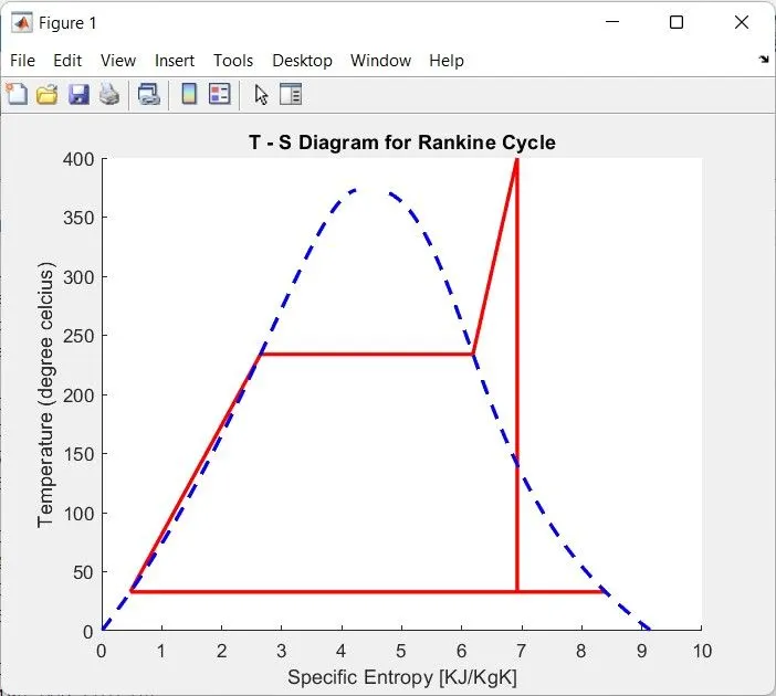
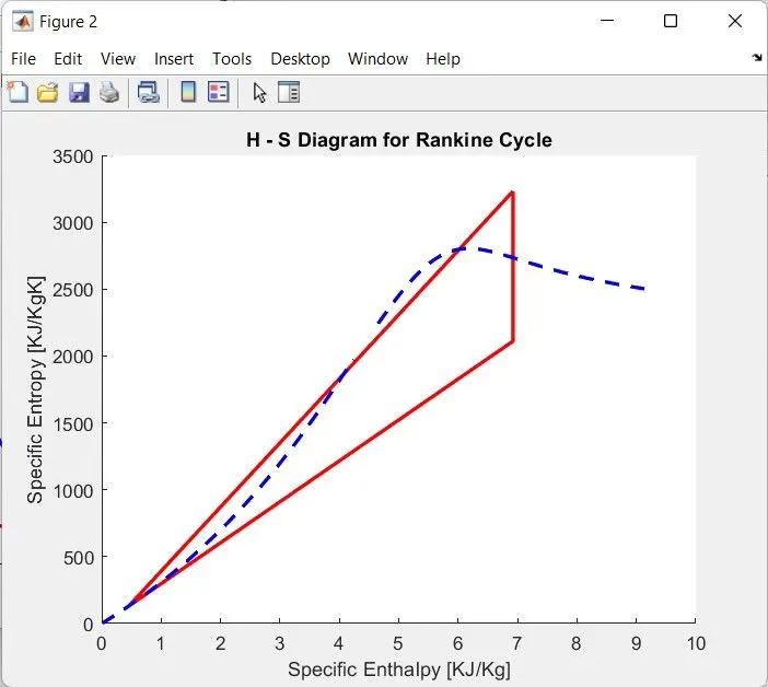
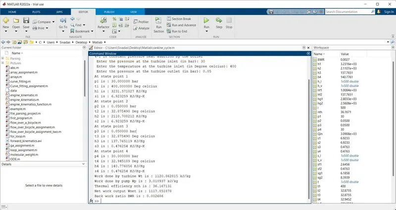
The T-S and H-S plots have been generated and the net work output and back work ratio are calculated

Net work output = 1117.85

Back work ratio = 0.002686

T - S diagram

H - S Diagram

Command window showing all the results

Conclusion

Using this program we can find various parameters of the rankine cycle for different input parameters. All the objectives we had at the begining of the project has also been completed.