Week 5 - Genetic Algorithm

A code in MATLAB to optimise the stalagmite function and find the global maxima of the function is given below:

First we need to create a function to assist us in writing the main code. The code to create that function is given below:

% Create a function of stalagmite
function [f] = stalagmite_func(input_vector)
x = input_vector(1);
y = input_vector(2);
f1x = (sin(5.1*pi*x+0.5))^6;
f1y = (sin(5.1*pi*y+0.5))^6;
f2x = exp(-4*log(2)*((x-0.0667)^2/0.64));
f2y = exp(-4*log(2)*((y-0.0667)^2/0.64));
f = -(f1x*f1y*f2x*f2y);
end

The main code to optimise the stalagmite function and find the global maxima of the function is given below:

% Stalagmite Mathematical Model

clear all
close all
clc

% Define the search space
x = linspace(0,0.6,150);
y = linspace(0,0.6,150);

% Create a 2D mesh
[xx, yy] = meshgrid(x,y);

num_cases=50;
tic

% Evaluating the stalagmite function
for i = 1:length(xx)
    for j = 1:length(yy)
        input_vector(1) = xx(i,j);
        input_vector(2) = yy(i,j);
        f(i,j) = stalagmite_func(input_vector);
    end
end

study_time = toc
figure(1)
surfc(xx,yy,-f);
shading interp
xlabel('x value')
ylabel('y value')
legend('X Values','Y values')
title('Stalagmite Function')

% Study 1 - Statistical behaviour
tic
for i = 1:num_cases
    [inputs,fopt1(i)] = ga(@stalagmite_func,2)
    xopt(i) = inputs(1);
    yopt(i) = inputs(2);
end
study_time1 = toc

figure(2)
subplot(2,1,1)
hold on
surfc(x,y,-f)
plot3(xopt,yopt,-fopt1,'Marker','o','MarkerSize',5,'MarkerFaceColor','r')
title('Unbounded inputs')
subplot(2,1,2)
plot(-fopt1)
shading interp
xlabel('Iteration')
ylabel('Function minimum')

% Study 2 - Statistical behaviour with upper and lower limits
tic
for i = 1:num_cases
    [inputs,fopt2(i)] = ga(@stalagmite_func,2,[],[],[],[],[0;0],[1;1]);
    xopt2(i) = inputs(1);
    yopt2(i) = inputs(2);
end
study_time2 = toc

figure(3)
subplot(2,1,1)
hold on
surfc(x,y,-f)
shading interp
plot3(xopt2,yopt2,-fopt2,'marker','o','MarkerSize',5,'MarkerFaceColor','r')
title('Bounded inputs')
subplot(2,1,2)
plot(-fopt2)
xlabel('Iterations')
ylabel('Function Minimum')

% Study 3 - Increasing GA iterations
options = optimoptions('ga');
options = optimoptions(options,'PopulationSize',170);

tic
for i = 1:num_cases
    [inputs,fopt3(i)] = ga(@stalagmite_func,2,[],[],[],[],[0;0],[1;1],[],[],options);
    xopt3(i) = inputs(1);
    yopt3(i) = inputs(2);
end
study_time3 = toc

figure(4)
subplot(2,1,1)
hold on
surfc(x,y,-f)
shading interp
plot3(xopt3,yopt3,-fopt3,'marker','o','MarkerSize',5,'MarkerFaceColor','r')
title('Bounded inputs modified population size')
subplot(2,1,2)
plot(-fopt3)
xlabel('Iterations')
ylabel('Function Maxima')

global_maxima = -fopt3

Explanation and Results

1. First we need to create the function code which would assist in writing the main code. So the equation we use here to create our function is the stagalmite function which is defined as:

f(x,y) = f1x * f1y * f2x *f2y, where

f1x = [sin(5.1*pi*x + 0.5)]^6

f1y = [sin(5.1*pi*y + 0.5)]^6

f2x = exp[-4ln(2) * (x-0.0667)^2/0.64]

f2y = exp[-4ln(2) * (y-0.0667)^2/0.64]

From the above, the global maxima can be calculated by

f(x,y) = -(f1x * f1y * f2x *f2y)

So based on the above equation, we write the function code. At first we start by using the 'function' syntax to define the function. Here we named our function as stalagmite_func. We save the file in the same name so as it work when the function is called.

2. Once the function is created, we write our main code by first giving it a heading by using '%' syntax followed by the usual commands such as clear all, close all and clc. After that we need to define our search space by using 'linspace' syntax.

x = linspace(0,0.6,150)

y = linspace(0,0.6,150)

3. After this we create a 2D mesh by using the 'meshgrid' syntax.

[xx, yy] = meshgrid(x,y)

4. After this we evaluate the stalagmite function by using the for loop syntax by taking the value i along the length of xx and j along the length of yy.

for i = 1:length(xx)

for j = 1:length(yy)

input_vector(1) = xx(i,j)

input_vector(2) = yy(i,j)

f(i,j) = stalagmite_func(input_vector)

end

end

After that we use the surfc syntax to create a three-dimensional surface plot with a contour plot underneath. We use the 'shading interp' syntax to dictate how the colors are shown for the existing datapoints. The plot for the stalagmite function we get is given below:

5. After this we need to go for study number 1 which is for unbounded and random inputs. We use for loop and take the value of i from 1:num_cases where num_cases is 50. Then we call the stalagmite function 'stalagmite_func' using the 'ga' syntax.

for i = 1:num_cases

[inputs,fopt1(i)] = ga(@stalagmite_func,2)

xopt(i) = inputs(1)

yopt(i) = inputs(2)

end

After this we use the subplot syntax, then surfc syntax to create a three-dimensional surface plot, and then the plot3 syntax for plotting xopt, yopt and fopt. Then we plot for fopt. We use shading_interp, then we label the x and y axis. The plot generated for this operation is given below:

Here the predictions are all over theplace due to randomness of the ga method we used.

6. After this we need to go for study number 2 which is for stalagmite function with statistical behaviour with upper and lower limits. We use for loop and take the value of i from 1:num_cases. But here while calling the function using ga syntax we also define the upper and lower limits inside the ga syntax.

for i = 1:num_cases

[inputs,fopt2(i)] = ga(@stalagmite_func,2,[],[],[],[],[0;0],[1;1])

xopt2(i) = inputs(1)

yopt2(i) = inputs(2)

end

We then create the subplots and plots the same way we created during study number 1. The plot thus generated is given below:

This has helped in narrowing the results for local maxima.

7. After this we need to go for study number 3 which is for stalagmite function with increasing GA iterations. Here we increase the population size from 50 to 170. We use for loop and take the value of i from 1:num_cases. But here while calling the function using ga syntax we also define the increase in population size inside the ga syntax.

for i = 1:num_cases

[inputs,fopt3(i)] = ga(@stalagmite_func,2,[],[],[],[],[0;0],[1;1],[],[],options);

xopt3(i) = inputs(1)

yopt3(i) = inputs(2)

end

We then create the subplots and plots the same way we created during study number 1. The plot thus generated is given below:

As you can see we are almost able to locate the global maxima.

The global maxima thus obtained is given below:

Concept of genetic algorithm

A genetic algorithm is a metaheuristic inspired by the process of natural selection that belongs to the larger class of evolutionary algorithms. Genetic algorithms are commonly used to generate high quality solutions to optimization and search problems. In genetic algorithm, a population of candidate solutions to an optimization problem is evolved towards better solutions. The genetic algorithm is a method for solving both constrained and unconstrained optimization problems that is based on natural selection, the process that drives biological evolution. The genetic algorithm repeatedly modifies a population of individual solutions. At each step, the genetic algorithm selects individuals from the current population to be parents and uses them to produce the children for the next generation. The genetic algorithm starts with a randomly generated population of size M. During the process of iteration, a new population of the same size is generated from the current population using three basic operations on the individuals of the population. Over successive generations, the population "evolves" toward an optimal solution. A GA proceeds to initialise a population of solutions and then to improvise it through repetitive application of the mutation, cross over, inversion and selection operators.

Ga syntax

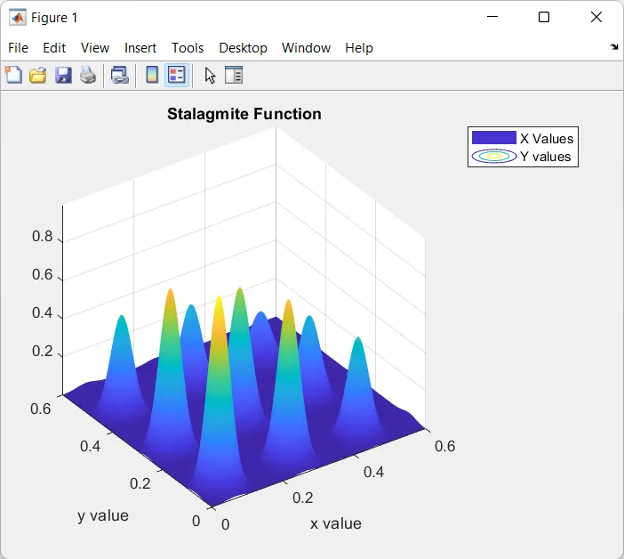
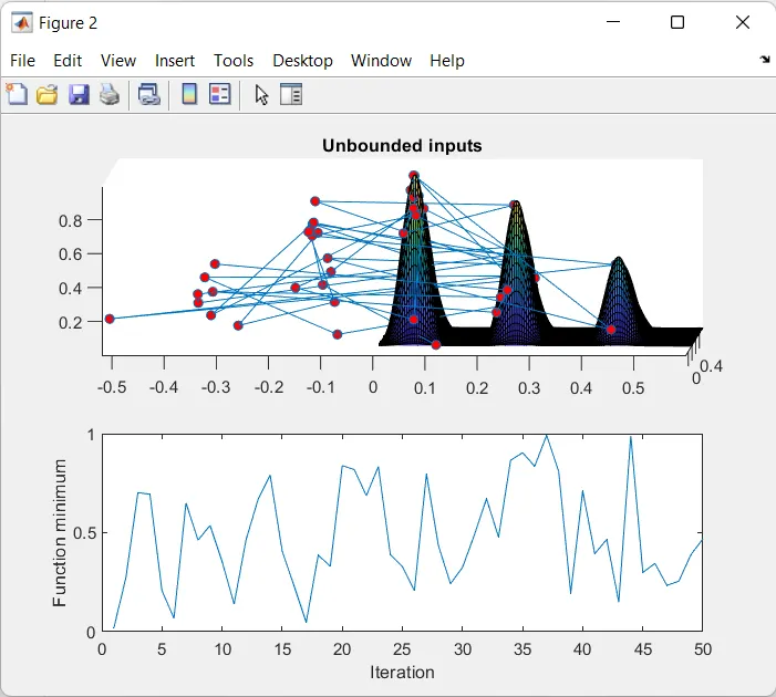
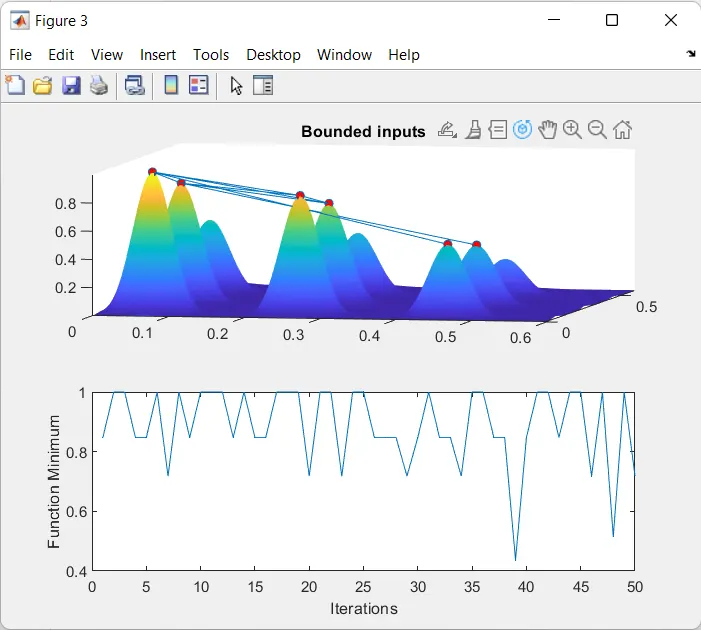
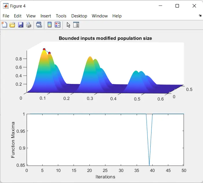
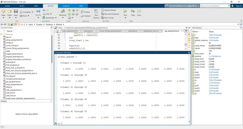
Ga function is used to find the minimum of the function using a genetic algorithm.

For Random Inputs:

x = ga(fun,nvars) finds a local unconstrained minimum, x, to the objective function, fun. nvars is the dimension (number of design variables) of fun.

For Bounded Inputs:

x = ga(fun,nvars,A,b,Aeq,beq,lb,ub) defines a set of lower and upper bounds on the design variables, x, so that a solution is found in the range lb ≤ x ≤ ub. (Set Aeq= [] and beq= [] if no linear equalities exist.)

For Population size:

x = ga(fun,nvars,A,b,[],[],lb,ub,nonlcon,IntCon,options) requires that the variables listed in IntCon take integer values.

where, Nvars – Number of Variables,

Aeq - linear equality constraints

beq – linear equality constraints

A – Linear inequality constraints

B – Linear inequality constraints

There were no major errors while programming.