Week 4.1 - Solving second order ODEs

A program that solves the ODE which represents the equation of motion of a simple pendulum with damping is written below.

First we create a function code which helps us in the creation of the main code is given below:

% Create a function 
function [dtheta_dt] = ode_func(t, theta, b, g, l, m)
theta1 = theta(1);
theta2 = theta(2);
dtheta1_dt = theta2;
dtheta2_dt = -(b/m)*theta2 - (g/l)*sin(theta1);
dtheta_dt = [dtheta1_dt ; dtheta2_dt];
end

The main code to solve the ODE is written below:

% Solve second order ODEs of simple pendulum

clear all
close all
clc

% Inputs given
l = 1;        % length of string in m
m = 1;        % mass in kg
b = 0.05;     % damping co-efficient
g = 9.81;     % acceleration due to gravity m/s^2

% Initial condition
theta_0 = [0;3];

% Time points
t_span = linspace(0,20,300);

% Solve ODE
[t,results] = ode45(@(t,theta)ode_func(t,theta,b,g,l,m),t_span,theta_0);

% Create a plot
figure(1)
plot(t,results(:,1),'LineWidth',1)
hold on
plot(t,results(:,2),'LineWidth',1)
axis([0 20 -6 8]);   
xlabel('time')
ylabel('plot')
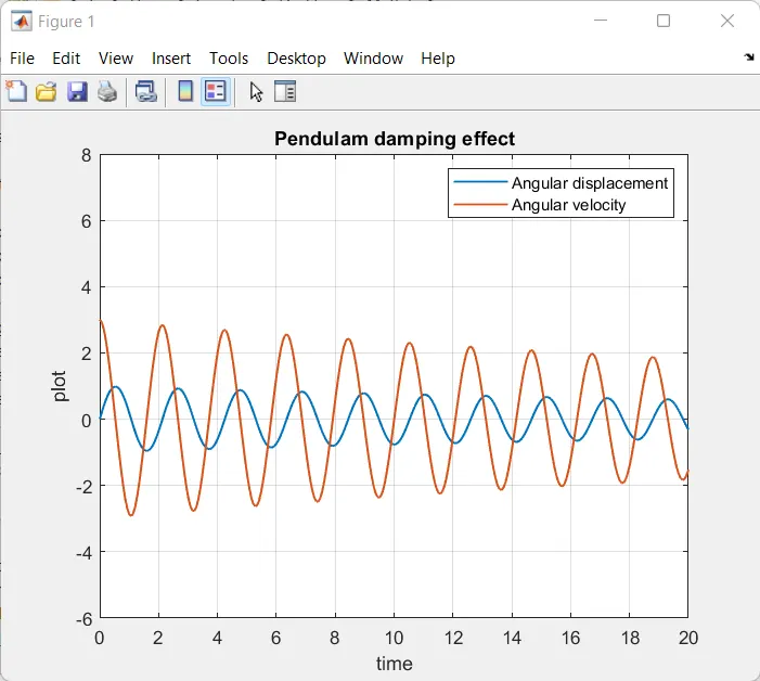
legend('Angular displacement','Angular velocity')
title('Pendulam damping effect')
grid on

% Create animation of the pendulam
ct = 1;
x0 = 0;
y0 = 0;
for i = 1:length(results)
    x1 = l*sin(results(i,1));
    y1 = -l*cos(results(i,1));
    figure(2)
    grid on
    plot(x1,y1,marker="o",MarkerSize=30,color='red')    % Pendulam ball
    hold on
    plot([x0 x1], [y0 y1], 'LineWidth',1,'Color','k')   % String
    plot([-1,1],[0,0], 'LineWidth',4,'Color','b')       % Base
    hold off
    axis([-2 2 -2 2])
    pause(0.1)
    M(ct) = getframe(gcf);
    ct = ct+1;
end

% Create an animation movie
movie(M)
videofile = VideoWriter('simple_pendulum.avi','uncompressed AVI');
open(videofile)
writeVideo(videofile,M)
close(videofile)

Explanation

1. The ODE equation for the pendulam to is given as:

d^2(theta)/dt^2 + (b/m)(dtheta/dt) + (g/l)sin(theta) = 0 ........(1)

Where, l = length of the movable rod

m = mass of pendulam bob

b = damping coefficient

We need to reduce the order of equation into lower order to solve this ODE

Let theta = theta1

d(theta)/dt = d(theta1)/dt = theta2 .......(2)

d^2(theta)/dt^2 = d^2(theta1)/dt^2 =d/dt(d(theta1)/dt) = d/dt(theta2) ..........(3)

Putting equation number (2) and (3) in (1), we get

d^2(theta1)/dt^2 +(b/m)(d(theta1)/dt) + (g/l)sin(theta1) = 0

d(theta2)/dt + (b/m)theta2 + (g/l)sin(theta1) = 0

Therefore,

d(theta2)/dt = -(b/m)theta2 - (g/l)sin(theta1)

2. Once we reduced the order of the equation, we develop a function to assist the main code with this equation. For that we create a function called 'ode_func' which consists of variables such as t, b, g, l, m, theta.

3. After creating the function, we write the main code starting with a heading using '%' syntax and then we write the usual commends such as clear all, close all and clc. After this we mention the input values given.

4. After this we define the initial condition of theta_0 = [0;3] which is the angular velocity. After this we define the time points t_span = linspace(0,20,300).

5. Now we solve the ODE by using the 'ode45' syntax, inside which we call the function 'ode_func', theta_0 and t_span.

6. Once it is solved, we need to plot the results using plot command. Two plots are plotted for angular velocity and angular displacement.

7. After this we need to create an animation which depicts the damping of the pendulam. So we take the initial postion of the pendulam as x0=0 and y0=0 and ct=1. Now we use a forloop to detemine the movement of the pendulam, where i = 1:length(results) and the subsequent x1 = l*sin(results(i,1)) and y1 = -l*cos(results(i,1)). Then we a plot graph for the pendulam ball using marker option, another plot for the string of the pendulam and another plot for the base. We define the axis and use 'getframe' syntax for movie animation. We close the for loop with ct = ct + 1 and then the 'end' syntax.

8. Finally we save the animation using the follwing code:

The animation created for the pendulam motion is given below:

https://www.youtube.com/watch?v=g-kmAHu6VWg

The errors faced during this are:

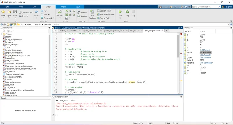
An addition parenthisis was added while calling the fuction which was sorted out after deleting it.