Project 2 - Rankine cycle Simulator
Aim: To create a Rankine cycle simulator using MATLAB
Objective:
- code used in the matlab should calculate the state points of the Rankine Cycle (any type of your choice) based on user inputs.
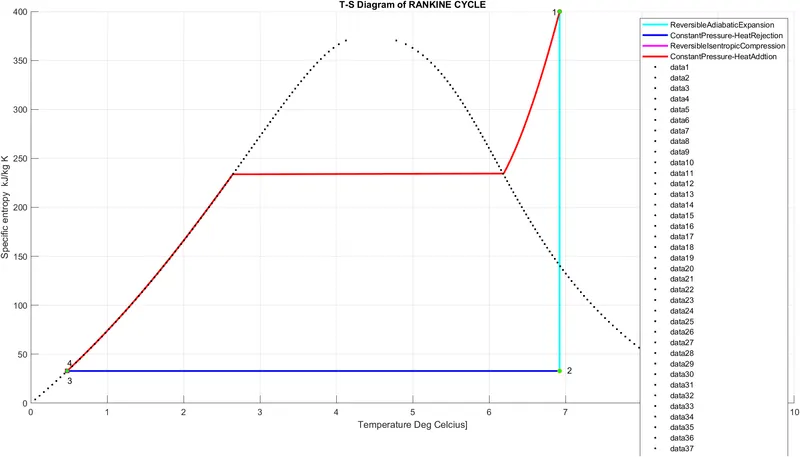
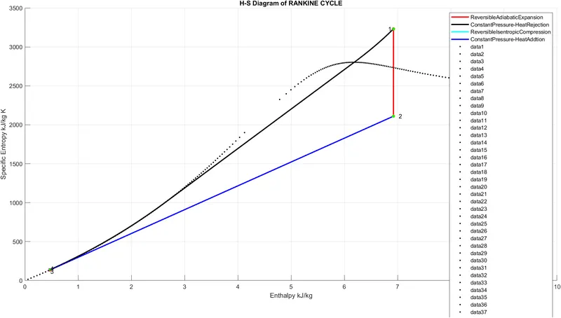
- Then, plot the corresponding T-s and h-s plots for the given set of inputs. Title and axes labels are a must, while legends could be used if necessary.
Rankine Cycle:
The Rankine cycle is an ideal cycle for vapour power cycle. In this cycle heat energy is supplied to the system via a boiler where the working fluid (typically water) is converted to a high pressure gaseous state (steam) in order to turn a turbine. After passing over the turbine the fluid is allowed to condense back into a liquid state as waste heat energy is rejected before being returned to boiler, completing the cycle. Friction losses throughout the system are often neglected for the purpose of simplifying calculations as such losses are usually much less significant than thermodynamic losses, especially in larger systems.
The Rankine cycle closely describes the process by which steam engines commonly found in thermal power generation plants harness the thermal energy of a fuel or other heat source to generate electricity. The ability of a Rankine engine to harness energy depends on the relative temperature difference between the heat source and heat sink. The greater the differential, the more mechanical power can be efficiently extracted out of heat energy, as per Carnot's theorem.
There are four processes in the Rankine cycle. The states are identified by numbers (in brown) in the T–s diagram.
- Process 1–2: The working fluid is pumped from low to high pressure. As the fluid is a liquid at this stage, the pump requires little input energy. Process 1-2 is isentropic compression.
- Process 2–3: The high-pressure liquid enters a boiler, where it is heated at constant pressure by an external heat source to become a dry saturated vapour. The input energy required can be easily calculated graphically, using an enthalpy–entropy chart (h–s chart, or Mollier diagram), or numerically, using steam tables or software. Process 2-3 is constant pressure heat addition in boiler.
- Process 3–4: The dry saturated vapour expands through a turbine, generating power. This decreases the temperature and pressure of the vapour, and some condensation may occur. The output in this process can be easily calculated using the chart or tables noted above. Process 3-4 is isentropic expansion.
- Process 4–1: The wet vapour then enters a condenser, where it is condensed at a constant pressure to become a saturated liquid. Process 4-1 is constant pressure heat rejection in condenser.
In an ideal Rankine cycle the pump and turbine would be isentropic, i.e., the pump and turbine would generate no entropy and hence maximize the net work output. Processes 1–2 and 3–4 would be represented by vertical lines on the T–s diagram and more closely resemble that of the Carnot cycle. The Rankine cycle shown here prevents the state of the working fluid from ending up in the superheated vapor region after the expansion in the turbine, which reduces the energy removed by the condensers.
CODE:
close all
clear all
clc
%% Heading and Process
fprintf('              RANKINE CYCLE SIMULATOR\n')
fprintf(' 1-2 is Isentropic Expansion in the Turbine \n')
fprintf(' 2-3 is Constant Pressure Heat Rejection by the Condenser \n')
fprintf(' 3-2 is Isentropic Compression in the Pump \n')
fprintf(' 4-1 is Constant Pressure Heat Addition by the Boiler\n\n')
%%  getting input variable from user
t1 = input('Enter the Temperature at the Turbine inlet T1(in Degree celsius): '); % getting Turbine inlet temperature
p1 = input('Enter the Pressure at the Turbine Inlet P1(in bar): ');               % getting Turbine inlet pressure
p2 = input('Enter the Pressure at the Turbine Outlet P2(in bar): ');              % getting Turbine outlet/ condenser inlet pressure
%% State variable at turbine
h1 = XSteam('h_pT',p1,t1); % Enthalpy with respect to pressure and temperature
s1 = XSteam('s_pT',p1,t1); % Specific entropy with respect to pressure and temperature
v1 = XSteam('v_pT',p1,t1); % Specific volume with respect to pressure and temperature
%% State variable at Conderser
s2 = s1;
h2 = XSteam('h_px',p2,XSteam('x_ps',p2,s2));
t2 = XSteam('T_ps',p2,s2);
v2 = XSteam('v_ps',p2,s2);
%% State variable at Pump Inlet
p3 = p2;
t3 = XSteam('Tsat_p',p3);
h3 = XSteam('hL_p',p3);
s3 = XSteam('sL_p',p3);
v3 = XSteam('vL_p',p3);
%% State variable at Boiler Inlet
s4 = s3;
p4 = p1;
h4 = XSteam('h_ps',p4,s4);
t4 = XSteam('T_ps',p4,s4);
v4 = XSteam('v_ps',p4,s4);
%% Plotting T-S Graph for Rankine cycle
figure(1)
hold on
plot([s1 s2],[t1 t2],'color','c','linewidth',2);
plot([s2 s3],[t2 t3],'color','b','linewidth',2);
plot([s3 s4],[t3 t4],'color','m','linewidth',2);
TempRange = linspace(t4,t1,500);
for i = 1:length(TempRange)
    s_range(i) = XSteam('s_pT',p1,TempRange(i));
    h_range23(i) = XSteam('h_ps',p1,s_range(i));
    h_range41(i) = XSteam('h_ps',p2,s_range(i));
end
plot(s_range,TempRange,'color','r','linewidth',2);
legend('ReversibleAdiabaticExpansion', 'ConstantPressure-HeatRejection', 'ReversibleIsentropicCompression', 'ConstantPressure-HeatAddtion');

%% Plotting H-S Graph for Rankine cycle.
figure(2)
hold on
plot([s1 s2],[h1 h2],'color','r','linewidth',2);
plot(s_range,h_range23,'color','k','linewidth',2);
plot([s3 s4],[h3 h4],'color','c','linewidth',2);
plot(s_range,h_range41,'color','b','linewidth',2);
legend('ReversibleAdiabaticExpansion', 'ConstantPressure-HeatRejection', 'ReversibleIsentropicCompression', 'ConstantPressure-HeatAddtion');

%% Plotting dry steam line in T-S graph
t_range = linspace(0,374.15,100);                   % Temperature from 0 to critical point of water in [degree C]
figure(1)
hold on
for i = 1:length(t_range)
    plot(XSteam('sL_t',t_range(i)),t_range(i),'.','color','k')
    plot(XSteam('sV_t',t_range(i)),t_range(i),'.','color','k')
end

%% Plotting dry steam line in H-S graph
figure(2)
hold on
for i = 1:length(t_range)
    plot(XSteam('sL_t',t_range(i)),XSteam('hL_t',t_range(i)),'.','color','k')
    plot(XSteam('sV_t',t_range(i)),XSteam('hV_t',t_range(i)),'.','color','k')
end

% Plotting state points in Rankine cycle T-S graph
figure(1)
hold on
plot(s1,t1,'o','MarkerFaceColor','g','MarkerSize',5)
text(s1-.1,t1-.5,'1')
plot(s2,t2,'o','MarkerFaceColor','g','MarkerSize',5)
text(s2+.1,t2+.5,'2')
plot(s3,t3,'s','MarkerFaceColor','r','MarkerSize',6)
text(s3,t3-10,'3')
plot(s4,t4,'o','MarkerFaceColor','g','MarkerSize',4)
text(s4,t4+8,'4')
grid on
title('T-S Diagram of RANKINE CYCLE')
xlabel('Temperature Deg Celcius]')
ylabel('Specific entropy  kJ/kg K')
saveas(figure(1),'T-S diagram.jpg');
% Ploting state points in Rankine cycle H-S graph
figure(2)
hold on
plot(s1,h1,'o','MarkerFaceColor','g','MarkerSize',5)
text(s1-0.1,h1-.5,'1')
plot(s2,h2,'o','MarkerFaceColor','g','MarkerSize',5)
text(s2+.1,h2+.5,'2')
plot(s3,h3,'s','MarkerFaceColor','r','MarkerSize',6)
text(s3,h3-20,'3')
plot(s4,h4,'o','MarkerFaceColor','g','MarkerSize',4)
text(s4,h4+15,'4')
grid on
title('H-S Diagram of RANKINE CYCLE')
xlabel('Enthalpy kJ/kg')
ylabel('Specific Entropy kJ/kg K')
saveas(figure(2),'H-S diagram.jpg');

%% Finally Calculating Work and Efficiency
Work_turbine = h1 - h2;                           % work out from turbine kJ/kg
Q_taken_out_condenser = h2 - h3;                  % heat rejected from condencer kJ/kg
Work_pump = h4 - h3;                              % work done by pump kJ/kg
Q_given_boiler = h1 - h4;                         % heat input kJ/kg
Back_Work_Ratio = Work_turbine / Work_pump;       % Back Work Ratio
SSE = 3600/(Work_turbine - Work_pump);            % Specific Steam Consumption in kg/kWh
Work_net = Work_turbine - Work_pump;              % Net work done
Effi_rankine = Work_net/Q_given_boiler;           % Rankine Cycle Efficiency
%% printing all the results
fprintf('\n                    RESULTS\n \n');
fprintf('At State point 1(Turbine):\n');
fprintf('Inlet Pressure of Turbine P1 is : %.2f Bar \n',p1);
fprintf('Inlet Temperature of Turbine T1 is : %.2f in Deg Celcius\n',t1);
fprintf('Inlet Enthalpy of Turbine H1 is : %.2f kJ/kg\n',h1);
fprintf('Inlet Specific Entropy of Turbine S1 is : %.2f in kJ/kg K\n \n',s1);

fprintf('At State Point 2(Condenser):\n');
fprintf('Inlet Pressure of Condensor P2 is : %.2f in Bar\n',p2);
fprintf('Inlet Temperature of Condenser T2 is : %.2f in Deg Celcius\n',t2);
fprintf('Inlet Enthalpy of Condenser H2 is : %.2f in kJ/kg\n',h2);
fprintf('Inlet Specific entropy of Condenser S2 is : %.2f in kJ/kg K\n \n',s2);

fprintf('At State Point 3(Pump):\n');
fprintf('Inlet Pressure of Pump P3 is : %.2f Bar\n',p3);
fprintf('Inlet Temperature of Pump T3 is : %.2f Deg Celcius\n',t3);
fprintf('Inlet Enthalpy of Pump H3 is : %.2f kJ/kg\n',h3);
fprintf('Inlet Specific entropy of Pump S3 ids : %.2f kJ/kg K\n \n',s3);

fprintf('At State Point 4(Boiler):\n');
fprintf('Inlet Pressure of Boiler P4 is : %.2f Bar\n',p4);
fprintf('Inlet Temperature of Boiler T1 is : %.2f Deg Celcius\n',t4);
fprintf('Inlet Enthalpy of Boiler H4 is : %.2f kJ/kg\n',h4);
fprintf('Inlet Specific entropy of Boiler S4 is : %.2f kJ/kg K\n \n',s4);

fprintf('Work and Efficiency of Rankine cycle:\n\n');
fprintf('Work done by Turbine WT is : %.2f kJ/kg\n',Work_turbine);
fprintf('Heat rejected from the Condenser Qr is : %.2f kJ/kg\n',Q_taken_out_condenser);
fprintf('Work done by Pump is : %.2f kJ/kg\n',Work_pump);
fprintf('Heat supplied to the Boiler  Qs is : %.2f kJ/kg\n \n',Q_given_boiler);

fprintf('Back Work Ratio BWR is : %.2f \n',Back_Work_Ratio);
fprintf('Specific Steam Consumption SSE is : %.2f kg/kWh \n',SSE);
fprintf('Net work Output of the Rankinecycle Wnet is : %.2f kJ/kg \n',Work_net);
fprintf('Efficiency of Rankine Cycle ETArankine is : %.2f %% \n',Effi_rankine*100)
CODE EXPLANATION:
1.Initially clear all contents like variables, vlaues and contents in the workspace and command window by using following command.
clear all: clear all the variables in the workspace
close all:deletes all figure including hose with hidden handles.
clc: clear command window
2. print the heading and process of the rankine cycle by using fprintf command
3. get the inputs such as turbine inlet temperature, turbine inlet pressure and turbine outlet pressure using input command
4. allot the input values to respective variable such as t1,p1 and p2 using equal to.
5. the enthalpy, specific entropy and volume at state 1 with respect given pressure and temperature is obtained using the XSteam function provided by skill lynk.
6. here h_pT represents enthalpy as a function of pressure and temperature, similerly same for s_pT and v_pT.
7. since dry saturated steam from the boiler (state 1) is expanded in the turbine isentropically (constant specific entropy)for developing mechanical work. s1 ie equal to s2.
8. then the enthalpy, temperature and volume is obtained using XSteam function.
9. by same method all the state points temperature, pressure, volume, enthalpy and specific entropy is obtained using Xsteam function.
10. the obtained data is plotted using figure command, plot command.
11. since the process 4 to 1 doesnot follows a straight path because the heat is supplied by the boiler to raise the temperature of water to saturated temperaure and again heated in the boiler to initial dry saturated liquid condition. The path is trased using for loop command.
12. the raise in temperature is split into number of points by using linspace command which evenly split the temperature point form one another.
13. then by using for loop all the specific entropy and enthalpy for different poits of temperature is found.
14. then T-S graph and H-S in the figure 1and figure 2 respectively is plotted with legend.
15. To plot dry steam line in T-S graph, the sL_T saturated liquid entropy and sV_T saturated vapour entropy with respect to temperature is plotted using plot command.
16. The same way the dry steam line in H-S graph the hL_T saturated liquid enthalpy and hV_T saturated vapour enthalpy with respect to respective saturated liquid and vapour entropy is plotted using plot command in figure 2.
17. then each state points are heighlited with green circle and denoted the state point using plot and text command.
18. the title of the graph is made with help of title command, the X and Y axis are labeled using xlabel and ylabel command.
19.then the figure is saved to jpg file using savesas command.
20.the same is repeated for figure 2.
21.the calculation for turbine work, pump work, heat added, heat removed, back work ratio, specific steam consuption, net work done and efficiency are done by arithmetic operators and values are given to respective variables.
22. using fprintf command the Rankine cycle simulator the output of all state points and needed values are displayed in the command window.
Output:
rankine cycle simulator
command window:
RANKINE CYCLE SIMULATOR
1-2 is Isentropic Expansion in the Turbine
2-3 is Constant Pressure Heat Rejection by the Condenser
3-2 is Isentropic Compression in the Pump
4-1 is Constant Pressure Heat Addition by the Boiler
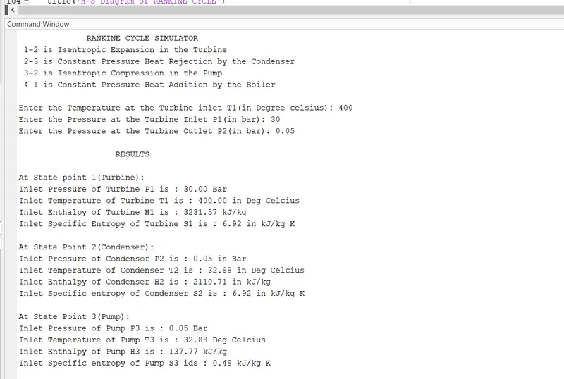
Enter the Temperature at the Turbine inlet T1(in Degree celsius): 400
Enter the Pressure at the Turbine Inlet P1(in bar): 30
Enter the Pressure at the Turbine Outlet P2(in bar): 0.05
RESULTS
At State point 1(Turbine):
Inlet Pressure of Turbine P1 is : 30.00 Bar
Inlet Temperature of Turbine T1 is : 400.00 in Deg Celcius
Inlet Enthalpy of Turbine H1 is : 3231.57 kJ/kg
Inlet Specific Entropy of Turbine S1 is : 6.92 in kJ/kg K
At State Point 2(Condenser):
Inlet Pressure of Condensor P2 is : 0.05 in Bar
Inlet Temperature of Condenser T2 is : 32.88 in Deg Celcius
Inlet Enthalpy of Condenser H2 is : 2110.71 in kJ/kg
Inlet Specific entropy of Condenser S2 is : 6.92 in kJ/kg K
At State Point 3(Pump):
Inlet Pressure of Pump P3 is : 0.05 Bar
Inlet Temperature of Pump T3 is : 32.88 Deg Celcius
Inlet Enthalpy of Pump H3 is : 137.77 kJ/kg
Inlet Specific entropy of Pump S3 ids : 0.48 kJ/kg K
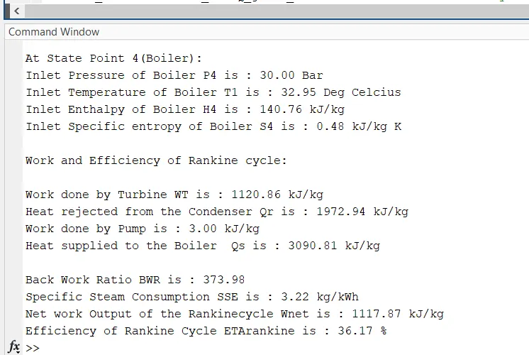
At State Point 4(Boiler):
Inlet Pressure of Boiler P4 is : 30.00 Bar
Inlet Temperature of Boiler T1 is : 32.95 Deg Celcius
Inlet Enthalpy of Boiler H4 is : 140.76 kJ/kg
Inlet Specific entropy of Boiler S4 is : 0.48 kJ/kg K
Work and Efficiency of Rankine cycle:
Work done by Turbine WT is : 1120.86 kJ/kg
Heat rejected from the Condenser Qr is : 1972.94 kJ/kg
Work done by Pump is : 3.00 kJ/kg
Heat supplied to the Boiler Qs is : 3090.81 kJ/kg
Back Work Ratio BWR is : 373.98
Specific Steam Consumption SSE is : 3.22 kg/kWh
Net work Output of the Rankinecycle Wnet is : 1117.87 kJ/kg
Efficiency of Rankine Cycle ETArankine is : 36.17 %
Thus output for the given input for the Rankine cycle is
- Net work output = 1117.87 kJ/kg
- Back work ratio = 373.98