Project 2 - Rankine cycle Simulator

PROJECT 2 - RANKINE CYCLE SIMULATOR 

AIM: To create a rankine cycle simulator and also, find the net work output and back work ratio at turbine inlet temperature and pressure of 400°C and 30 bars and turbine outlet pressure of 0.05bar

THEORY:

1) The Rankine cycle or Rankine Vapor Cycle is the process widely used by power plants such as coal-fired power plants or nuclear reactors. In this mechanism, a fuel is used to produce heat within a boiler, converting water into steam which then expands through a turbine producing useful work. This is a thermodynamic cycle which converts heat into mechanical energy—which usually gets transformed into electricity by electrical generation.

2) The Rankine cycle operates in the following steps: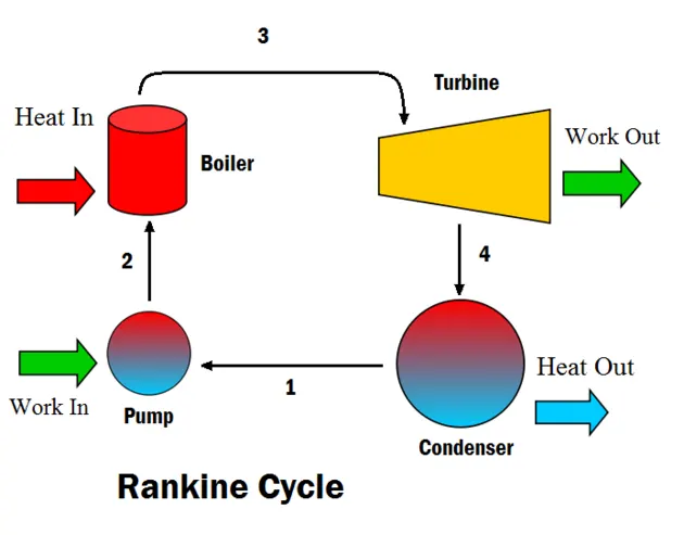

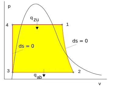
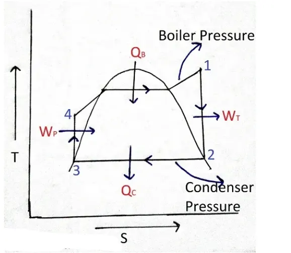
• Process 3-4:First, the working fluid (water) is enter the pump at state 3 at saturated liquid and it is pumped (ideally isentropically) from low pressure to high (operating) pressure of boiler by a pump to the state 4. During this isentropic compression water temperature is slightly increased. Pumping requires a power input (for example, mechanical or electrical). The conservation of energy relation for pump is given as
  Wpump = m (h4 - h3)

• Process 4-1:The high pressure compressed liquid enters a boiler at state 4 where it is heated at constant pressure by an external heat source to become a saturated vapour at statel’which in turn superheated to state 1 through super heater. Common heat source for power plant systems are coal (or other chemical energy), natural gas, or nuclear power. The conservation of energy relation for boiler is given as
  Qin =m (h1 - h4)

• Process 1 –2:The superheated vapour enter the turbine at state 1 and expands through a turbine to generate power output. Ideally, this expansion is isentropic. This decreases the temperature and pressure of the vapour at state 2. The conservation of energy relation for turbine is given as
  Wturbine = m (h1 –h2)

• Process 2 –3:The vapour then enters a condenser at state 2. At this state, steam is a saturated liquid-vapour mixture where it is cooled to become a saturated liquid at state 3. This liquid then re-enters the pump and the cycle is repeated. The conservation of energy relation for condenser is given as
  Qout = m (h2 –h3)

3) The net work done is calculated as follows;
Pump work input:
Wpump,in = v1(P2-P2)

Turbine work output:
Wturb,out = h3 - h4

Hence, the net work output of the ideal cycle is
Wnet,out = wturb,out - wpump,in

4)The back work ratio BWR is calculated as follows;
Back work ratio = Compressor work/Turbine work = (h4-h3)/(h2-h1)

PROCEDURE:

1) Below is the code used for calculating and plotting the requirements;

%Rankine Cycle
clear al
close all
clc

disp('                               RANKINE CYCLE                                ');
disp('1-2 is Isentropic Expansion in the Turbine');
disp('2-3 is Constant Pressure Heat rejection by the Condensor');
disp('3-4 is Isentropic Expansion in the Pump');
disp('4-1 is Constant Pressure Heat addition to the Boiler'); 

%Inputs:
disp('                               INPUTS                                  ');
p1 = input('Enter the Pressure at turbine inlet(bars):');
T1 = input('Enter the Temperature at the Turbine inlet(degree C):');
p2 = input('Enter the Pressure at the Condenser(bars):');

%Using the XSteam functions,the enthalpy and entropy at various
%points can be calculated:

%Taking data from Xsteam file at point 1:
h1 = XSteam('h_pT', p1, T1);
s1 = XSteam('s_pT', p1, T1); 

%Taking data from Xsteam file at point 2:    
s2 = s1;
%For Dryness factor s2 = sf2 + x(sfg)
sf2 = XSteam('sL_p',p2);
sg2 = XSteam('sV_p',p2); 
sfg2 = sg2-sf2;
 
if(s2<=sg2)
    x2 = (s2-sf2)/(sfg2);
else
    x2 = 1;
end 
 
Ts2 = XSteam('Tsat_p',p2);
 
if (x2<1)
    T2 = Ts2;
else
    % s2 = sg2+CpV2*(log(T2/Ts2))
    % CpV_p Saturated vapour heat capacity
    CpV2 = XSteam('CpV_p',p2); 
    %(log(T2/Ts2)) = (s2-sg2)/CpV2
    % T2/Ts2 = exp((s2-sg2)/CpV2)
    % T2 = Ts2 * exp((s2-sg2)/CpV2)
    % add 273.15 to convert tempreture unit from degree Celsius to Kelvin
    T_2 = (Ts2+273.15)*exp((s2-sg2)/CpV2);
    T2 = T_2-273.15;
end
 
x2 = (s2-sf2)/(sfg2);
hf2 = XSteam('hL_p',p2);
hg2 = XSteam('hV_p',p2);
hfg2 = hg2-hf2;
%h2 = XSteam('h_ps',p2,s2);
if (x2<1)
    h2 = hf2 + x2*hfg2;
else
    h2 = hg2 + CpV2*(T2-Ts2);
end

%Taking data from Xsteam file at point 3:
p3 = p2;
h3 = hf2;
s3 = sf2;
T3 = Ts2;

%Taking data from Xsteam file at point 4:

p4 = p1;
s4 = s3;

v3 = XSteam('vL_p',p3);
W_p = v3*(p4-p3)*100;
h4 = h3 + Wp;
 
 
% s4 = sf4-cpL4*log(Ts4/T4)
sf4 = XSteam('sL_p',p4);
Ts4 = XSteam('Tsat_p',p4);
CpL4 = XSteam('CpL_p',p4);
% log(Ts4/T4)=(sf4-s4)/CpL4
% Ts4/T4 = exp((sf4-s4)/CpL4)
T4 = Ts4/(exp((sf4-s4)/CpL4));
%Other data for saturater liquid and vapour
T6 = XSteam('Tsat_p', p1);          % Saturated Temperature at Pressure 1
s5 = XSteam('sL_p', p1);            % Saturated Liquid entropy at pressure 1
s6 = XSteam('sV_p', p1);            % Saturated Vapour entropy at Pressure 1
h5 = XSteam('hL_p', p1);            % Saturated Liquid Enthalpy at Pressure 1
h6 = XSteam('hV_p', p1);            % Saturated Vapour Enthalpy at pressure 1
T5 = T6;

%Calculating the Entropy and Enthapy at the saturation curve:

Temp = linspace(0,500,600);

for i = 1:length(Temp)

sv(i) = XSteam('sV_T',Temp(i));
sl(i) = XSteam('sL_T',Temp(i));

hv(i) = XSteam('hV_T', Temp(i));
hl(i) = XSteam('hL_T', Temp(i));

end

%Calculating Net Work Output(W_net):

W_t = h1-h2;
W_net = W_t-W_p;

%Calculating Back Work Ratio:
Bw_ratio = W_p/W_t;

%Calculating the Thermal efficiency:
Q_in = h1-h4;
thermal_eff = (W_net/Q_in)*100;

%Calculating Specific Steam Consumption:
% wkt 1J = 3600kg/s
SSC = 3600/W_net;

% Displaying Results in the command window:
disp('                       Results                       ');
disp('At stage point 1');
n1 = sprintf('P1 is %.3f bar',p1);
disp(n1);
n2 = sprintf('T1 is %.3f C',T1);
disp(n2);
n3 = sprintf('h1 is %.3f kJ/kg',h1);
disp(n3);
n4 = sprintf('s1 is %.3f kJ/kgK',s1);
disp(n4);
disp('At stage point 2');
n11 = sprintf('P2 is %.3f bar',p2);
disp(n11);
n21 = sprintf('T2 is %.3f C',T2);
disp(n21);
n31 = sprintf('h2 is %.3f kJ/kg',h2);
disp(n31);
n41 = sprintf('s2 is %.3f kJ/kgK',s2);
disp(n41);
disp('At stage point 3');
n12 = sprintf('P3 is %.3f bar',p3);
disp(n12);
n22 = sprintf('T3 is %.3f C',T3);
disp(n22);
n32 = sprintf('h3 is %.3f kJ/kg',h3);
disp(n32);
n42 = sprintf('s3 is %.3f kJ/kgK',s3);
disp(n42);
disp('At stage point 4');
n13 = sprintf('P4 is %.3f bar',p4);
disp(n13);
n23 = sprintf('T4 is %.3f C',T4);
disp(n23);
n33 = sprintf('h4 is %.3f kJ/kg',h4);
disp(n33);
n43 = sprintf('s4 is %.3f kJ/kgK',s4);
disp(n43);
n14 = sprintf('W_t is %.3f kJ/kg',W_t);
disp(n14);
n15 = sprintf('W_p is %.3f kJ/kg',W_p);
disp(n15);
n16 = sprintf('Net work ouput is %.3f kJ/kg',W_net);
disp(n16);
n17 = sprintf('Thermal efficiency is %.2f Percent',thermal_eff);
disp(n17);
n18 = sprintf('Specific steam consumption is %.2f kg/kWh',SSC);
disp(n18);
n19=sprintf('Back work ratio is %.4f ',Bw_ratio);
disp(n19);

%Plotting for Saturation Line
T = linspace(1,560,1000);
for i = 1:length(T)
    sf(i) = XSteam('sL_T' ,T(i));   % Saturated Liquid Entropy
    sg(i) = XSteam('sV_T' ,T(i));   % Saturated Vapour Entropy
    hf(i) = XSteam('hL_T' ,T(i));   % Saturated Liquid Enthalpy
    hg(i) = XSteam('hV_T' ,T(i));   % Saturated Vapour Enthalpy
    
end
figure(1)
hold on
plot(sf,T,'color','g','linestyle','--','linewidth',1)
plot(sg,T,'color','g','linestyle','--','linewidth',1)
plot([s1 s2],[T1 T2], 'color', 'r', 'linewidth',1)
plot([s2 s3],[T2 T3], 'color', 'r', 'linewidth',1)
plot([s3 s4],[T3 T4], 'color', 'r', 'linewidth',1)
plot([s4 s5],[T4 T5], 'color', 'r', 'linewidth',1)
plot([s5 s6],[T5 T6], 'color', 'r', 'linewidth',1)
s_1 = linspace(s6,s1,1000);
for j = 1:length(s_1)
    Tc(j) = XSteam('T_ps',p1,s_1(j));
end
plot(s_1,Tc,'color','r','linewidth',1)
text(s1+0.1, T1, '1')
text(s2+0.1, T2, '2')
text(s3, T3-20, '3')
text(s4, T4+20, '4')
title('Temperature Vs Entropy')
xlabel('Entropy (Kj/kg-k)')
ylabel('Temeperature (Deg. Celcius)')
legend('Saturation Curve')

% Plotting H-S Diagram for Rankine Cycle
figure(2)
% enthalpy vs entropy
figure(2)
figure(2)
hold on
plot(sf,hf,'color','g','linestyle','--','linewidth',1)
plot(sg,hg,'color','g','linestyle','--','linewidth',1)
plot([s1 s2],[h1 h2],'color','r','linewidth',1)
plot([s2 s3],[h2 h3],'color','r','linewidth',1)
plot([s3 s4],[h3 h4],'color','r','linewidth',1)
hc = linspace(h4,h5,100);
for k = 1:length(hc)
    s_c(k) = XSteam('s_ph',p1,hc(k));
end
plot(s_c,hc,'color','r','linewidth',1)
plot([s5 s6],[h5 h6],'color','r','linewidth',1)
for l = 1:length(s_1)
    h_c(l) = XSteam('h_ps',p1,s_1(l));
end
plot(s_1,h_c,'color','r','linewidth',1)
text(s1+0.1,h1,'1')
text(s2+0.1,h2,'2')
text(s3,h3-100,'3')
text(s4,h4+200,'4')
title('Enthalpy Vs Entropy')
xlabel('Entropy (Kj/kg-k)')
ylabel('Enthalpy (KJ/Kg)')
legend('Saturation Curve')

CODE EXPLANATION:

1) Here we use input command to take user input for turbine inlet pressure and temperature as well as the condenser inlet pressure.

2) From the inputs we can find the properties such as enthalpy and entropy of the point 1 by using Xsteam file similar to the steam table.

3) As we know point 1 to point 2 isentropic expansion we know the value of entropy at point 2. So using this info and also the condenser pressure, we calculate other properties such as enthalpy and temperature. Also we calculate the dryness fraction by checking the temperature is less than or equal to saturated temperated at that point.
If temperature is less than the saturated temperature then dryness fraction is calculated to get the actual value of enthalpy.

4) For properties at point 3 we know that the process 2-3 is isobaric heat rejection. So we know that the point 3 is completely saturated liquid state, so we get enthalpy and entropy for this point which is equal to the hf2 i.e the saturated liquid enthalpy of point 2. 
The properties at point 3 will help us determine the excess heat.

5) Process 3-4 is isentropic compression that means entropy at point 4 is equal that of point 3. Also process 4-1 is isobaric heat addition process, so pressure at point 4 is equal to point 1. To calculate the enthalpy we use the Wp i.e pump work corelation. 

6) The saturated liquid and vapour enthalpy and entropy at point 1 is also calculated.

7) To plot the graph we make use of the values acquired from the above procedure.

8) Also to calculate the efficiency and BWR respective formulas are used to calculate them.

OUTPUT:

1) Below shown is the command window output;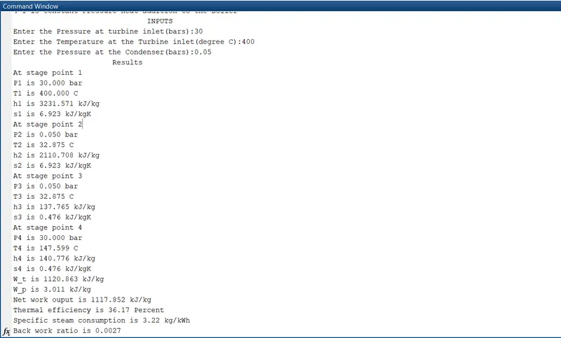

2) The required H-S diagram and T-S diagram are plotted as shown below;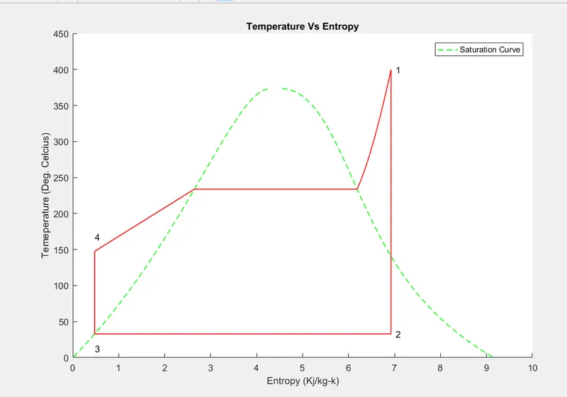

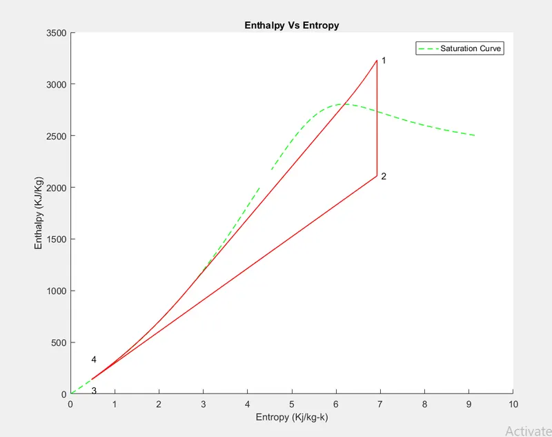
CONCLUSION AND LEARNING OUTCOME:

• We learned how to plot a rankine cycle using matlab programming for the given input.
• Xsteam is used like steam table in matlab program.