Project 2 - Rankine cycle Simulator

AIM:

Creation of Rankine cycle simulator from given input and reading the data from standard thermodynamic library of steam table.

OBJECTIVE:

• To create a Rankine Cycle simulator in MATLAB.
• To calculate the state point using function XSteam.
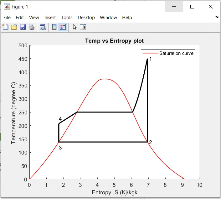
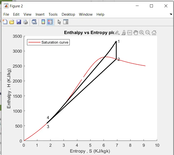
• To plot the T-S and H-S curve for given input in Rankine Cycle.
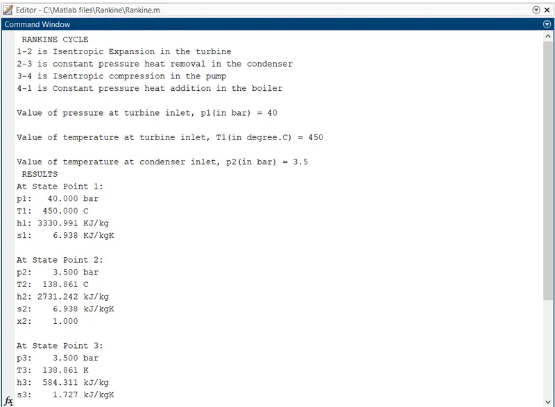
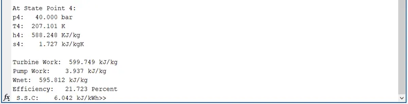
• To get output in the command window for each state point in cycle.

THEORY:

RANKINE CYCLE:

The Rankine cycle or Rankine Vapor Cycle is the process widely used by power plants such as coal-fired power plants or nuclear reactors. In this mechanism, a fuel is used to produce heat within a boiler, converting water into steam which then expands through a turbine producing useful work.

In a Rankine cycle, high-pressure liquid water (1) enters a boiler where it is heated to saturation temperature (2), vaporized, and superheated (3). The superheated steam is fed to a turbine, where it expands and generates mechanical work. The steam exits the turbine at a lower pressure and temperature as either superheated steam or steam with a vapor quality (4). After the steam is condensed (5), a pump compresses the liquid water to high pressure (1). Select “P-H diagram” to see the cycle on a pressure-enthalpy diagram. Use sliders to select the inlet pressure to the turbine P₃ and one of four outlet pressures P₄. Use a slider to vary the turbine efficiency η_T, which is the ratio of work produced by the turbine to the work produced by a reversible turbine between the same inlet and outlet pressures. The irreversible turbine pathway (η_T < 1) is the dashed black line on the P-H diagram; the reversible turbine pathway is the orange dashed line. Select “Rankine cycle” to view a schematic of the cycle, and select “turbine” to show the inlet and outlet conditions for the turbine and the work generated

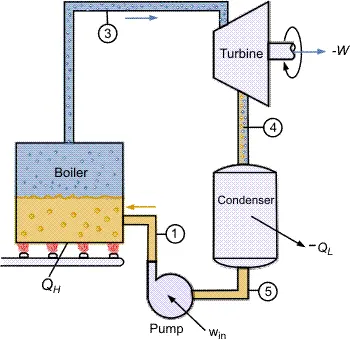
PROCESSES:

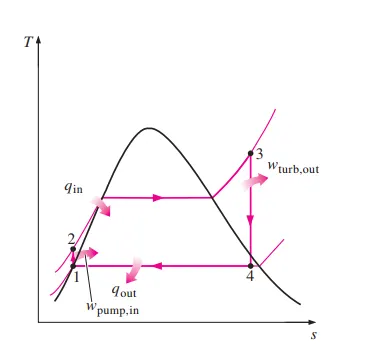
Process 1–2: The working fluid is pumped from low to high pressure. As the fluid is a liquid at this stage, the pump requires little input energy. Process 1-2 is isentropic compression.

Process 2–3: The high-pressure liquid enters a boiler, where it is heated at constant pressure by an external heat source to become a dry saturated vapor. The input energy required can be easily calculated graphically, using an enthalpy-entropy chart (H-S CHART) OR (MOLLIER DIAGRAM), or numerically, using Steam tables or software. Process 2-3 is constant pressure heat addition in the boiler.

Process 3–4: The dry saturated vapor expands through a Turbine, generating power. This decreases the temperature and pressure of the vapor, and some condensation may occur. The output in this process can be easily calculated using the chart or tables noted above. Process 3-4 is isentropic expansion.

Process 4–1: The wet vapor then enters a Condensor, where it is condensed at a constant pressure to become a Saturated liquid. Process 4-1 is constant pressure heat rejection in the condenser.

MATLAB PROGRAM:

%% Rankine Cycle Simulator 
%Objective of this program is to simulate the rankine cycle 
%Plotting t-s and h-s diagram using data from XSteam data
%Water and steam properties according to IAPWS IF-97  
clear all
close all
clc

%%
disp(' RANKINE CYCLE ');                                    % Displaying
disp('1-2 is Isentropic Expansion in the turbine');
disp('2-3 is constant pressure heat removal in the condenser');
disp('3-4 is Isentropic compression in the pump');
disp('4-1 is Constant pressure heat addition in the boiler');

%%
%Obtaining the input data
p1 = input('\nValue of pressure at turbine inlet, p1(in bar) = ');
T1 = input('\nValue of temperature at turbine inlet, T1(in degree.C) = ');
p2 = input('\nValue of temperature at condenser inlet, p2(in bar) = ');
%% 
% Extracting data _ defining variables
% State 1
h1 = XSteam('h_pT', p1, T1);        % extracting enthalpy at state pt 1
s1 = XSteam('s_pT', p1, T1);        % similarly

% State 2
s2 = s1;                            % Isentropic expansion                
sf2= XSteam('sL_p', p2);            % Saturated liquid Entropy
sg2 = XSteam('sV_p', p2);           % Saturated Vapour Entropy
x2 = (s2-sf2)/(sg2-sf2);
hf2 = XSteam('hL_p', p2);           
hg2 = XSteam('hV_p', p2);
h2 = hf2 + (x2*(hg2-hf2));

% State 3
p3 = p2;                            % Constant pressure Heat rejection in condenser
s3= XSteam('sL_p', p3);
h3 = XSteam('hL_p', p3);

% State 4
s4 = s3;
p4 = p1;
%%
% Work done by turbine
Wt = h1 - h2;

% Work done to run pump
v3 = XSteam('vL_p', p3);
Wp = v3*(p4 - p3)*100;
h4 = h3 + Wp;

%net work
Wnet = Wt - Wp;

%Heat into the system
Qin = h1 - h4;

%Heat out of the system
Qout = h2 - h3;

%Thermal efficiency
eff = (Wnet/Qin)*100;

%Specific Steam Consumption
%SSC = mass flow rate/power
SSC = (3600/Wnet);

%%
%Calculating temperatures at the state points
T3 = XSteam('Tsat_p', p3);
T2 = T3;
Cp4 = XSteam('Cp_ps', p4, s4);
Cv4 = XSteam('Cv_ps', p4, s4);
k = Cp4/Cv4;
T4 = T3/((p3/p4)^((k-1)/k));

%Calculating temperature, entropy and enthalpy at the vapour and liquid
%line for plotting
T6 = XSteam('Tsat_p', p1);
s5 = XSteam('sL_p', p1);
s6 = XSteam('sV_p', p1);
h5 = XSteam('hL_p', p1);
h6 = XSteam('hV_p', p1);
T5 = T6;

%%
%Plotting the saturation curve
T = linspace(1,375,1000);
for i = 1:length(T)

sf(i) = XSteam('sL_T', T(i));
sg(i) = XSteam('sV_T', T(i));
hf(i) = XSteam('hL_T', T(i));
hg(i) = XSteam('hV_T', T(i));
end

%Plotting T-s diagram
figure(1)
hold on
plot(sf, T, 'r','linewidth',1)
plot(sg, T, 'r','linewidth',1)
plot([s1 s2], [T1 T2], 'k', 'linewidth', 2)
plot([s2 s3], [T2 T3] ,'k', 'linewidth', 2)
plot([s3 s4], [T3 T4], 'k', 'linewidth', 2)
plot([s4 s5], [T4 T5], 'k', 'linewidth', 2)
plot([s5 s6], [T5 T6], 'k', 'linewidth', 2)
sc1 = linspace(s6, s1, 1000);
for l = 1:length(sc1)
 Tc1(l) = XSteam('T_ps', p1, sc1(l));
end
plot(sc1, Tc1, 'k', 'linewidth', 2)
text(s1+0.1, T1, '1')
text(s2+0.1, T2, '2')
text(s3, T3-20, '3')
text(s4, T4+20, '4')
title('Temp vs Entropy plot')
xlabel('Entropy ,S (Kj/kgk')
ylabel('Temperature (degree C) ')
legend('Saturation curve')


%%
%Plotting h-s diagram
figure(2)
hold on
plot(sf, hf, 'r', 'linewidth', 1)
plot(sg, hg, 'r',  'linewidth', 1)
plot([s1 s2], [h1 h2], 'k', 'linewidth', 2)
plot([s2 s3], [h2 h3], 'k', 'linewidth', 2)
plot([s3 s4], [h3 h4], 'k', 'linewidth', 2)
hc = linspace(h4, h5, 100);
for k = 1:length(hc)
sch(k) = XSteam('s_ph', p1, hc(k));
end
plot(sch,hc, 'k', 'linewidth', 2)
plot([s5 s6], [h5 h6], 'k', 'linewidth', 2)
for m = 1:length(sc1)
hc1(m) = XSteam('h_ps', p1, sc1(m));
end
plot(sc1, hc1, 'k', 'linewidth', 2)
text(s1+0.1, h1, '1')
text(s2+0.1, h2, '2')
text(s3, h3-100, '3')
text(s4, h4 +200, '4')
title('Enthalpy vs Entropy plot')
xlabel('Entropy , S (KJ/kgk) ')
ylabel('Enthalpy , H (KJ/kg)')
legend('Saturation curve','location','northwest')


%%
% Displaying Results
disp(' RESULTS');
fprintf('At State Point 1:\n');
fprintf('p1: %8.3f bar\n', p1);
fprintf('T1: %8.3f C\n', T1);
fprintf('h1: %8.3f KJ/kg\n', h1);
fprintf('s1: %8.3f KJ/kgK\n\n', s1);
fprintf('At State Point 2:\n');
fprintf('p2: %8.3f bar\n', p2);
fprintf('T2: %8.3f C\n', T2);
fprintf('h2: %8.3f kJ/kg\n', h2);
fprintf('s2: %8.3f kJ/kgK\n', s2);
fprintf('x2: %8.3f\n\n', x2);
fprintf('At State Point 3:\n');
fprintf('p3: %8.3f bar\n', p3);
fprintf('T3: %8.3f K\n', T3);
fprintf('h3: %8.3f kJ/kg\n', h3);
fprintf('s3: %8.3f kJ/kgK\n\n', s3);
fprintf('At State Point 4:\n');
fprintf('p4: %8.3f bar\n', p4);
fprintf('T4: %8.3f K\n', T4);
fprintf('h4: %8.3f KJ/kg\n', h4);
fprintf('s4: %8.3f kJ/kgK\n\n', s4);
fprintf('Turbine Work: %8.3f kJ/kg\n', Wt);
fprintf('Pump Work: %8.3f kJ/kg\n', Wp);
fprintf('Wnet: %8.3f kJ/kg\n', Wnet);
fprintf('Efficiency: %8.3f Percent \n ', eff);
fprintf('S.S.C: %8.3f kJ/kWh', SSC);

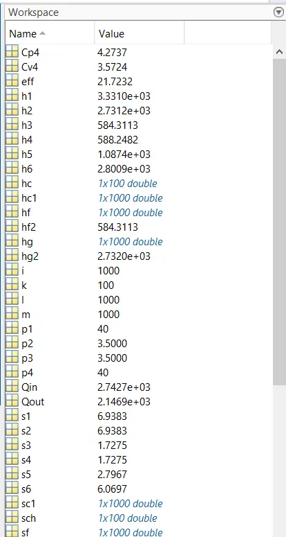
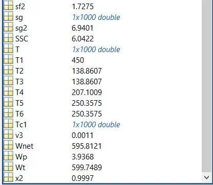
Workspace:

RESULTS:

[T vs S ] & [ H vs S ] plots :

RESULT IN COMMAND WINDOW:

CONCLUSION:

Thus the Rankine cycle simulator is obtained using MATLAB by writing simple code where the values are extracted using 'XSteam' steam table and the result is obtained for the given values of input.