Project 2 - Rankine cycle Simulator

Project 2: To understand the concept of Rankine cycle by referring to standard thermal engineering text book and to create a Rankine Cycle Simulator using MATLAB.

• The code should calculate the state points of the Rankine Cycle (any type of your choice) based on user inputs.
• Then, plot the corresponding T-s and h-s plots for the given set of inputs.

Required Inputs:

Turbine Inlet temperature = 400° C

Turbine Inlet Pressure = 30 bars

Turbine Outlet Pressure = 0.05 bars = Condenser Inlet Pressure

Calculate the followings,

• Net work output
• Back work ratio

Ideal Rankine Cycle:

The Simple Ideal Rankine Cycle consists of the following four thermodynamic processes:

• 1-2 : Isentropic expansion in turbine.
• 2-3 : Isobaric heat rejection in condenser.
• 3-4 : Isoentropic compression in feed pump.
• 4-1 : Isobaric heat addition in boiler.

As depicted into the following figure:

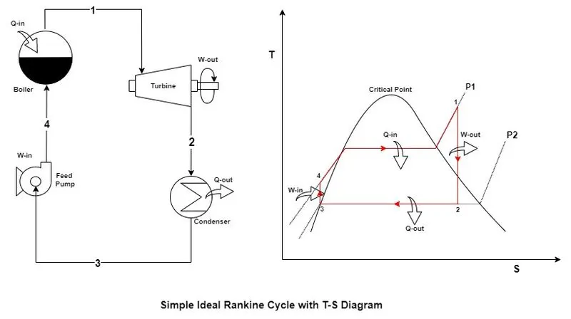
High pressure superheated vapour enters into the turbine (1) where it expands to do work till the vapour pressure and temperature drops to the condenser pressure. Then it enters to the condenser (2) where the saturated vapours get condensed to the saturated liquid at the condenser pressure. Then the saturated liquid enters into boiler feed pump(3),which increases its pressure to the level of boiler working pressure and feeds it into the boiler water drum (4). In the boiler the high pressure liquid water is heated till gets superheated till the desired temperature. Then again high pressure superheated steam is supplied to the turbine(1) and cycle repeats.

The Energy Analysis is done using Strady Flow Energy Equation for per unit mass of steam. Neglecting the smaller terms the following relations are obtained. Where symbols have their usual meanings.

The workdone by turbine is `w_t = h_2 - h_1` .

The heat rejected in condenser is `q_"out" = h_3 - h_2`.

The workdone by feed pump is `w_p = h_4 - h_3 = v (P_4 - P_3)`.

The heat added in the boiler is `q_"in" = h_1 - h_4`.

Thus, The networkdone is given as `w_"net" = w_t - w_p`.

The Back Work Ration is given as `BWR = frac{w_p}{w_t}` .

The Thermal efficinecy of the system is given as `eta_"therm" = frac{w_"net"}{q_"in"}`.

The Specific Steam Consumption is given as `SSC = 3600/w_"net"`.

Steps to write a code for Rankine Cycle Simulator:

• The XSteam file has been copied to the working directory where the Rankine simulator program code will be written.
• Read the XSteam file for its usage into the program code and to get familiar with the XSteam functions to get various water and steam properties.
• The code has been started with the commands to close all previously open plots , to clear work space and to clean command window.
• The required inputs have been given to the simulator program with the help of code.
• Prior to that the process identification printed out.
• Then the saturation temperatures for boiler working pressure and condenser pressure have been evaluated with the help of XSteam library functions.
• Similarly using respective XSteam functions the specific entalpy and specific entropy for saturated liquid and saturated vapour are evaluated.
• By the same way the properties at all the state points are evaluated using XSteam functions and calculated using functional relationships if required.
• The points on the saturated liquid line and saturated vapour line along with the critical point are evaluated using for loop and respective XSteam functions.
• Similarly the points on the heating curve of compressed liquid till the saturation temperature and heating curve for the superheated region are obtained using for and if loops as required.
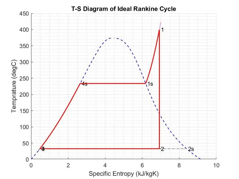
• The T-S diagram has been plotted by using required data obtained earlier.
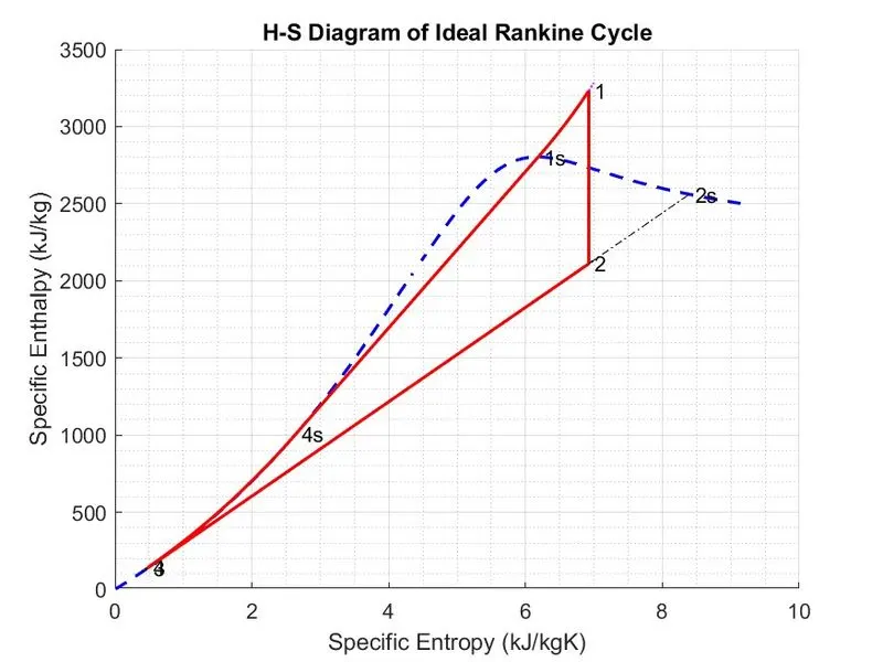
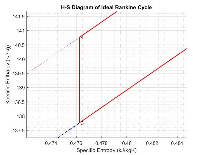
• Similarly the H-S diagram has been plotted.
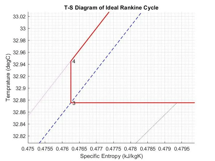
• In both the diagrams the points 3 & 4 are indistinguishable due to the scale of the diagram, for more clarity the exagerated views of the same are obtained and presented here which show that the temperature and enthalpy rise while pumping is very less as compared to the temperature and enthalpy scales of the respective diagrams.
• The thermal efficiency along with back work ratio and specific steam consumption are calculated.
• The required outputs have been printed into the command window.

Rankine Cycle Simulator Code:

%Rankine Cycle Simulator
clear all;
close all;
clc;

% Processes in the ideal Rankine Cycle
fprintf('\t\t\t RANKINE CYCLE SIMULATOR \n\n');
fprintf('1-2  Isentropic Expansion in the Turbine\n');
fprintf('2-3  Constant Pressure Heat Rejection in the Condenser\n')
fprintf('3-2  Isentropic Compression in the Pump\n')
fprintf('4-1  Constant Pressure Heat Addition by the Boiler\n\n')

% Input arguments
P1 = input('Enter the Pressure at the Turbine Inlet (in bar): ');
T1 = input('Enter the Temperature at the Turbine inlet (in Degree celsius): ');
P2 = input('Enter the Pressure at the Condenser (in bar): ');

fprintf('\t\t\t RESULTS \n');

% Calculation of Saturation Temperature at P1 & P2
Tsat_P1=XSteam('Tsat_p',P1);
Tsat_P2=XSteam('Tsat_p',P2);

if (T1 < Tsat_P1)
    sprintf('Error: System cannot have steam of Temperature %3.f degC at Turbine inlet for %3.f bar of working Pressure',T1,P1)
else    

% Calculation of Enthalpy & Entropy of saturated vapour at P1 
Hg_1=XSteam('hV_p',P1);
Sg_1=XSteam('sV_p',P1);
% Calculation of Enthalpy & Entropy of saturated vapour at P2
Hg_2=XSteam('hV_p',P2);
Sg_2=XSteam('sV_p',P2);
% Calculation of Enthalpy & Entropy of saturated liquid at P2
Hf_2=XSteam('hL_p',P2);
Sf_2=XSteam('sL_p',P2);
% Calculation of Enthalpy & Entropy of saturated liquid at P1
Hf_1=XSteam('hL_p',P1);
Sf_1=XSteam('sL_p',P1);

% Calculation of Process properties at state 1
fprintf('At State point 1- Turbine inlet \n');
fprintf('P1 is : %f bar \n',P1);
fprintf('T1 is : %f degC \n',T1);
H1=XSteam('h_pT',P1,T1);
fprintf('H1 is : %f kJ/kg \n',H1);
S1=XSteam('s_pT',P1,T1);
fprintf('S1 is : %f kJ/kgK \n\n',S1);

% Calculation of Process properties at state 2
fprintf('At state point 2-Turbine Outlet(Condenser Inlet)\n');
fprintf('P2 is : %f bar \n', P2);
S2 = S1;
fprintf('S2 is : %f kJ/kgK \n', S2);

%Calculating value of X
if(S2 < Sg_2)
    X2 = (S2 - Sf_2) / (Sg_2 - Sf_2);   % Dryness Fraction at state point 2
else
    X2=1;    
end
fprintf('X2 is : %f \n', X2);

%calculating value of T2 & H2
if(X2 < 1)
    T2=Tsat_P2;
    H2 = Hf_2 - X2 * (Hf_2 - Hg_2);
else 
    T2=XSteam('T_ps',P2,S2);
    H2=XSteam('h_pT',P2,T2);
end    

fprintf('T2 is : %f degC \n', T2)   
fprintf('H2 is : %f kJ/kg \n', H2)

%Calculation of Dryness fraction from Volume fraction (Alternate Way just to verify)
steamfrac =XSteam('vx_ps',P2,S2);                        % Steam volume fraction
specvol =XSteam('v_ps',P2,S2);                           % Specific volume 
Vfg = XSteam('vV_p',P2) - XSteam('vL_p',P2);             % Difference between specific volume of saturated liquid and saturated vapour phase at P2 
DF= (steamfrac*specvol/Vfg);                             % Calculating Dryness fraction by volume fraction method
fprintf('Dryness Fraction (DF) by volume fraction method is : %f  \n\n', DF) % Printing Drayness fraction 

% Calculation of Process properties at state 3
fprintf('At state point 3 - Consenser Outlet(Feed Pump Inlet)\n')
P3 = P2;
fprintf('P3 is : %f bar \n', P3)
V3 = XSteam('vL_p', P3);
T3 = Tsat_P2;                    % No subcooling of liquid (Saturated Liquid)
fprintf('T3 is : %f degC \n', T3)
H3 =Hf_2;
fprintf('H3 is : %f kJ/kg \n', H3)
S3 =Sf_2;
fprintf('S3 is : %f kJ/kgK \n\n', S3)

% Calculation of Process properties at state 4
fprintf('At state point 4- Boiler Inlet(Feed Pump Outlet) \n')
P4 = P1;
fprintf('P4 is : %f bar \n', P4)
S4 = S3;
fprintf('S4 is : %f kJ/kgK \n', S4)
Wp = V3 * (P4 - P3) * 100;
H4 = Wp + H3;
fprintf('H4 is : %f kJ/kg \n', H4)
T4=XSteam('T_ps',P4,S4);
fprintf('T4 is : %f degC \n\n', T4)

% Finding points for plotting saturation Liquid and Vapour lines 
temp = linspace(0,(T1+100), 1000);
for i = 1 : length(temp)
     H_L(i) = XSteam('hL_T', temp(i));
     H_V(i) = XSteam('hV_T', temp(i));
     S_L(i) = XSteam('sL_T', temp(i));
     S_V(i) = XSteam('sV_T', temp(i));
end

% Finding points on the Constant pressure curves for P1 and P2 for specified entropy range
NTP = linspace(0.4,7,500);
for j = 1:length(NTP)
    TP1(j) = XSteam('T_ps',P1,NTP(j));
    TP2(j) = XSteam('T_ps',P2,NTP(j));
    HP1(j) = XSteam('h_ps',P1,NTP(j));
    HP2(j) = XSteam('h_ps',P2,NTP(j));
end   

% Finding points on heating curve of the compressed liquid at constant pressure, till the saturation temperature
NTPL = linspace(S4,Sf_1,100);
for k = 1:length(NTPL)
    TSPL(k) = XSteam('T_ps',P1,NTPL(k));
    HSPL(k) = XSteam('h_ps',P1,NTPL(k));
end   

% Finding points on the Constant Pressure heating curve at P1 for Superheated region
NTP1 = linspace(Sg_1,S1,500);
for y = 1:length(NTP1)
    TSP1(y) = XSteam('T_ps',P1,NTP1(y));
    HSP1(y) = XSteam('h_ps',P1,NTP1(y));
end

% Finding points on the Constant Pressure heating curve at P2 for Superheated region  
if S2>Sg_2
    NTP2 = linspace(Sg_2,S2,500);
  for z= 1:length(NTP2)
    TSP2(z) = XSteam('T_ps',P2,NTP2(z));
    HSP2(z) = XSteam('h_ps',P2,NTP2(z));
  end
end

% Plotting T-s Plot
figure(1)
hold on
plot(S_L, temp, 'b', 'linestyle','--','linewidth', 1)      % Plotting Saturated liquid line
plot(S_V, temp, 'b', 'linestyle','--','linewidth', 1)      % Plotting Saturated Vapour line  
plot(NTP,TP1,'Color','m','LineStyle',':','LineWidth',1);   % Plotting Constant Pressure line for P1
plot(NTP,TP2,'Color','k','LineStyle',':','LineWidth',1);   % Plotting Constant Pressure line for P2

plot([S1 S2], [T1 T2], 'r', 'linewidth', 1.5)            % Plotting Isentropic expansion in Turbine   
text(S1,T1,' 1')                                         % Marking State Point 1 for turbine inlet
text(S2,T2,' 2')                                         % Marking State Point 2 for turbine outlet
text(Sg_2,Tsat_P2,' 2s')                                 % Marking Projection of point 2 on Saturated vapour line i.e. 2s

if S2 > Sg_2                                             % Plotting line between State point 2 & 2s with if condition 
    plot(NTP2,TSP2,'Color','r','linewidth', 1.5)         % Plots for superheated region
    plot([Sg_2 S3], [Tsat_P2 T3], 'r', 'linewidth', 1.5)
else
    plot([S2 Sg_2], [T2 Tsat_P2],'Color','k','lineStyle','-.', 'linewidth', 0.5) % Plots for Saturated & Wet region
    plot([S2 S3], [T2 T3], 'r', 'linewidth', 1.5)
end

text(S3,T3,' 3')                                            % Marking State point 3 for Feed pump inlet
plot([S3 S4], [T3 T4], 'r', 'linewidth', 1.5)               % Plotting isentropic compression in pump (Compressed liquid)
text((S4),T4,' 4')                                          % Marking State Point 4 for Feed pump outlet
plot(NTPL,TSPL,'Color','r','LineWidth',1.5);                % Plotting heating of compressed liquid till the saturation point 4s
text(Sf_1,Tsat_P1,' 4s')                                    % Marking Saturated liquid point for heating at P1
plot([Sf_1 Sg_1], [Tsat_P1 Tsat_P1], 'r', 'linewidth', 1.5) % Plotting Constant Pressure heating curve for phase change region where Temp also remains constant
text(Sg_1,Tsat_P1,' 1s')                                    % Marking Saturated vapour point for constant pressure heating at P1 
plot(NTP1,TSP1,'r', 'linewidth', 1.5)                       % Plotting constant pressure heating curve for superheated region

title('T-S Diagram of Ideal Rankine Cycle')                 % Plot Title  
ylabel('Temprature (degC)')                                 % Y axis label 
xlabel('Specific Entropy (kJ/kgK)')                         % X axis label
grid on       
grid minor
saveas(gcf,'T-S Diagram Ideal Rankine Cycle','jpg');

% Plotting H-S Plot
figure(2)
hold on
plot(S_L, H_L, 'b','linestyle','--', 'linewidth', 1.5)     % Plotting Saturated liquid line
plot(S_V, H_V, 'b','linestyle','--', 'linewidth', 1.5)     % Plotting Saturated vapour line
plot(NTP,HP1,'Color','m','LineStyle',':','LineWidth',1);   % Plotting Constant Pressure line for P1
plot(NTP,HP2,'Color','k','LineStyle',':','LineWidth',1);   % Plotting Constant Pressure line for P2

plot([S1 S2], [H1 H2], 'r', 'linewidth', 1.5)              % Plotting Isentropic expansion in Turbine
text(S1,H1,' 1')                                           % Marking State point 1 for turbine inlet
text(S2,H2,' 2')                                           % Marking State point 2 for turbine outlet    
text(Sg_2,Hg_2,' 2s')                                      % Marking Projection of point 2 on Saturated vapour line i.e. 2s

if S2 > Sg_2                                               % Plotting line between State point 2 & 2s with if condition 
    plot(NTP2,HSP2,'Color','r','linewidth', 1.5)           % Plots for superheated region
    plot([Sg_2 S3], [Hg_2 H3], 'r', 'linewidth', 1.5)
else
    plot([S2 Sg_2], [H2 Hg_2],'Color','k','lineStyle','-.', 'linewidth', 0.5) % Plots for Saturated & Wet region
    plot([S2 S3], [H2 H3], 'r', 'linewidth', 1.5)
end
text(S3,H3,' 3')                                           % Marking State point 3 for Feed pump inlet
plot([S3 S4], [H3 H4], 'r', 'linewidth', 1.5)              % Plotting isentropic compression in pump (Compressed liquid)
text(S4,H4,' 4')                                           % Marking State point 4 for Feed pump outlet
plot(NTPL,HSPL,'Color','r','LineWidth',1.5);               % Plotting heating of compressed liquid till the saturation point 4s
text(Sf_1,Hf_1,' 4s')                                      % Marking Saturated liquid point for heating at P1
plot([Sf_1 Sg_1], [Hf_1 Hg_1], 'r', 'linewidth', 1.5)      % Plotting Constant Pressure heating curve for phase change region where Temp also remains constant
text(Sg_1,Hg_1,' 1s')                                      % Marking Saturated vapour point for constant pressure heating at P1
plot(NTP1,HSP1,'Color','r','LineWidth',1.5);               % Plotting constant pressure heating curve for superheated region

title('H-S Diagram of Ideal Rankine Cycle')                % Plot Title
ylabel('Specific Enthalpy (kJ/kg)')                        % Y axis label
xlabel('Specific Entropy (kJ/kgK)')                        % X axis label
grid on
grid minor
saveas(gcf,'H-S Diagram Ideal Rankine Cycle','jpg');

% Work done, heat, SSC and efficiency calculations
Wt = H1 - H2;                                              % Calculating Workdone by turbine
fprintf('Workdone by turbine is : %f kJ/kg \n', Wt)            % Printing Workdone by turbine 
fprintf('Workdone by pump is : %f kJ/kg \n', Wp)               % Printing Workdone by Feed Pump
Wnet = Wt - Wp;                                            % Calculating Net Work done
fprintf('Net Workdone is : %f kJ/kg \n', Wnet)             % Printing Net Workdone
BWR = Wp/Wt;                                               % Calculating Back Work ratio 
fprintf('Back Work Ratio is: %f \n',BWR)                   % Printing Back Work Ratio
Qin = H1 - H4;                                             % Calculating Heat Supplied by boiler  
thermal_eff = Wnet/ Qin ;                                  % Calculating Thermal Efficiency
fprintf('Thermal efficiency is : %f \n', thermal_eff);     % Printing Thermal efficeincy
SSC = 3600 / Wt;                                           % Calculating Specific steam consuption
fprintf('S.S.C is : %f kg/kWh \n', SSC)                    % Printing Specific Steam Consumption

end

The output in the command window with required inputs are as below:

			 RANKINE CYCLE SIMULATOR 

1-2  Isentropic Expansion in the Turbine
2-3  Constant Pressure Heat Rejection in the Condenser
3-2  Isentropic Compression in the Pump
4-1  Constant Pressure Heat Addition by the Boiler

Enter the Pressure at the Turbine Inlet (in bar): 30
Enter the Temperature at the Turbine inlet (in Degree celsius): 400
Enter the Pressure at the Condenser (in bar): 0.05
			 RESULTS 
At State point 1- Turbine inlet 
P1 is : 30.000000 bar 
T1 is : 400.000000 degC 
H1 is : 3231.571027 kJ/kg 
S1 is : 6.923259 kJ/kgK 

At state point 2-Turbine Outlet(Condenser Inlet)
P2 is : 0.050000 bar 
S2 is : 6.923259 kJ/kgK 
X2 is : 0.814256 
T2 is : 32.875490 degC 
H2 is : 2110.708212 kJ/kg 
Dryness Fraction (DF) by volume fraction method is : 0.814285  

At state point 3 - Consenser Outlet(Feed Pump Inlet)
P3 is : 0.050000 bar 
T3 is : 32.875490 degC 
H3 is : 137.765119 kJ/kg 
S3 is : 0.476254 kJ/kgK 

At state point 4- Boiler Inlet(Feed Pump Outlet) 
P4 is : 30.000000 bar 
S4 is : 0.476254 kJ/kgK 
H4 is : 140.776056 kJ/kg 
T4 is : 32.945189 degC 

Workdone by turbine is : 1120.862815 kJ/kg 
Workdone by pump is : 3.010937 kJ/kg 
Net Workdone is : 1117.851878 kJ/kg 
Back Work Ratio is: 0.002686 
Thermal efficiency is : 0.361671 
S.S.C is : 3.211811 kg/kWh 
>> 

T-S Diagram:

	T-S Diagram
	Exagerated View for State point 3 & 4

H-S Diagram:

	H-S Diagram
	Exagerated View for State point 3 & 4

Conclusion:

Thus the Rankine Cycle Simulator is created using MATLAB and successfully tested for required inputs.