Project 2 - Rankine cycle Simulator

Main Code:

clear all
close all
clc

% Creating Rankine cycle Simulator
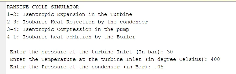
disp('RANKINE CYCLE SIMULATOR')
disp('1-2: Isentropic Expansion in the Turbine')
disp('2-3: Isobaric Heat Rejection by the condenser')
disp('3-4: Isentropic Compression in the pump')
disp('4-1: Isobaric heat addition by the Boiler')
disp(' ') % finding the states

t=linspace(0,373.15,300);

% Inputs to be specified
P1=input(' Enter the pressure at the turbine Inlet (In bar): ');
T1=input(' Enter the Temperature at the turbine Inlet (in degree Celsius): ');
P2=input(' Enter the Pressure at the condenser (in Bar): ');
disp(' ') % Finding the states

% We need two independent, intensitive properties to define any state

% Inlet of the Turbine / State point 1(P,T)
h1=XSteam('h_pT',P1,T1); % h_pT Entalpy as afunction of pressure and temperature
s1=XSteam('s_pT',P1,T1); % s_pT Specific entropy as afunction of pressure and temperature
h_l1=XSteam('hL_p',P1);  % Enthalpy at Liquid state
h_g1=XSteam('hV_p',P1);  % Enthalpy at gaseous state
s_l1=XSteam('sL_p',P1);  % Entropy at Liquid state
s_g1=XSteam('sV_p',P1);  % Entropy at gaseous state
T_sat1=XSteam('Tsat_p',P1);


% Inlet of the condenser State point 2(p,s)
s2=s1;
s_l2=XSteam('sL_p',P2);
s_g2=XSteam('sV_p',P2);

% Dryness Fraction
X=(s2-s_l2)/(s_g2-s_l2);

h_l2=XSteam('hL_p',P2); % enthalpy at liquid state
h_g2=XSteam('hV_p',P2); % enthalpy at gaseous state
h2=h_l2+X*(h_g2-h_l2);
T2=XSteam('T_ph',P2,h2);
T_sat2=XSteam('Tsat_p',P2);

%  Exit of the condenser / State Point 3(p,)
% Wet vapour (2 pahse mixture)is converted to satuarated liquid
h3=h_l2;
s3=s_l2;
P3=P2; % Isobaric process
T3=T2;

% State point 4(p,s)
s4=s3;
P4=P1; % Isentopic process
h4=XSteam('h_ps',P4,s4);
T4=XSteam('T_ps',P4,s4);

%Plotting

% T-S diagram
figure(1),clf
hold on

% Saturation curve
for i=1:length(t)
    plot(XSteam('sL_T',t(i)),t(i),'r.')
    plot(XSteam('sV_T',t(i)),t(i),'r.')
end

% Rankine cycle
plot([s1 s2],[T1 T2],'linewidth',2,'color','g')
text(s1,T1,'1','FontSize',15)

% Beyond saturation curve
if X > 1
    T3=T_sat2;
    plot([s2 s_g2 s3 s4],[T2 T_sat2 T3 T4],'linewidth',2,'color','g')
    text(s1,T2,'2','Fontsize',15)
    text(s3,T3,'3','Fontsize',15,'HorizontalAlignment','left','VerticalAlignment','top')
    % Beneath Saturation curve
else
    plot([s2 s3 s4],[T2 T3 T4],'linewidth',2,'color','g')
    text(s1,T2,'2','Fontsize',15)
    text(s3,T3,'3','Fontsize',15,'HorizontalAlignment','left','VerticalAlignment','top')
end

n=linspace(T1,T2,500);
for i=1:length(n)
    plot(XSteam('s_pT',P1,n(i)),n(i),'.','linewidth',2,'color','g')
end

plot([s_l1 s_g1],[T_sat1 T_sat1],'linewidth',2,'color','g')
text(s_l1,T_sat1,'4','Fontsize',15,'VerticalAlignment','bottom')
xlabel('Entropy(kJ/kg-k)')
ylabel('Temperature(k)')
title('T-S Diagram')

% h-s Diagram
figure(2),clf
hold on

% Saturation curve
for i=1:length(t)
    plot(XSteam('sL_T',t(i)),XSteam('hL_T',t(i)),'r.')
    plot(XSteam('sV_T',t(i)),XSteam('hV_T',t(i)),'r.')
end

% Rankine cycle
plot([s1 s2 s3 s4 s1],[h1 h2 h3 h4 h1 ],'Linestyle','--','linewidth',1,'color','b')
text(s1,h1,'1','Fontsize',15)
text(s2,h2,'2','Fontsize',15)
text(s3,h3,'3','Fontsize',15)
text(s4,h4+90,'4','Fontsize',15)
xlabel('Entropy(KJ/kg-K)')
ylabel('Enthalpy(KJ/kg)')
title('h-s Diagram')

% Calculation of desired quantities
% Work done by Turbine
W_t=h1-h2;

% Work done by Pump
W_p=h4-h3;

% Net work done
W_net=W_t-W_p;

% Thermal efficiency
n_thermal=(1-((h2-h3)/(h1-h4)))*100;

% Back work ratio
BWR=W_p/W_t;

% Spcific steam conductivity
SSC=3600/W_t;

% Displaying results in command window
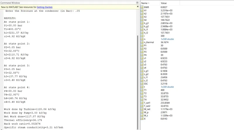
disp('RESULTS:')

disp('At state point 1:')
fprintf('P1=%.2f bar\n',P1)
fprintf(['T1=%.2f' char(176) 'C\n'],T1)
fprintf('h1=%.2f KJ/kg\n',h1)
fprintf('s1=%.2f KJ/kgK\n',s1)
disp(' ')

disp('At state point 2:')
fprintf('P2=%.2f bar\n',P2)
fprintf(['T2=%.2f' char(176) 'C\n'],T2)
fprintf('h2=%.2f KJ/kg\n',h2)
fprintf('s2=%.2f KJ/kgK\n',s2)
disp(' ')


disp('At state point 3: ')
fprintf('P3=%.2f bar\n',P3)
fprintf(['T3=%.2f' char(176) 'C\n'],T3)
fprintf('h3=%.2f KJ/kg\n',h3)
fprintf('s3=%.2f KJ/kgK\n',s3)
disp(' ')


disp('At state point 4: ')
fprintf('P4=%.2f bar\n',P4)
fprintf(['T4=%.2f' char(176) 'C\n'],T4)
fprintf('h4=%.2f KJ/kg\n',h4)
fprintf('s4=%.2f KJ/kgK\n',s4)
disp(' ')

fprintf('Work done by Turbine=%.2f kJ/kg\n',W_t)
fprintf('Work done by Pump=%.2f kJ/kg\n',W_p)
fprintf('Net Work done=%.2f KJ/kg\n',W_net)
fprintf('Thernal efficiency=%.2f%%\n',n_thermal)
fprintf('Back work ratio=%f\n',BWR)
fprintf('Specific steam conductivity=%.2f kJ/kwh\n',SSC)

CODE EXPLANATION:

• Initiall the platform for filling required inputs is established.
• It is followed by specifying all state point variables from Xsteam library.
• we need at least 2 independent, insensitive properties to define any state.
• during phase changes, the temperature remains constant.
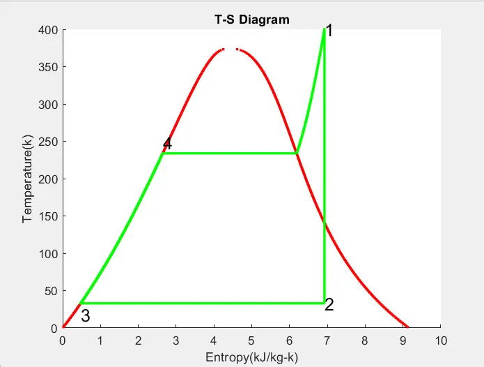
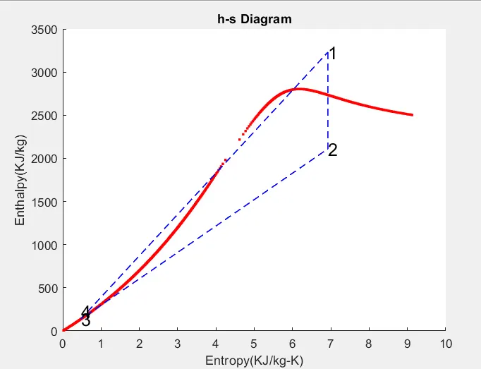
• The T-s and h-s diagrams are ploted contaiing the Rankine cycle and the saturation curve.
• calculate the efficiency,net work,back work ratio and display it in the command window.
• My states 3 and 4 are mixed up because in the 3 to 4 process entropy remains constant and Temperature T3 and T4 are almost the same which means that the pump work is very small.

RESULTS:

PLOTS:

CONCLUSION:

• The Rankine cycle is a most practical and power generating cycle.
• Superheating increase the thermal efficiency of the cycle.