Project 2 - Rankine cycle Simulator
AIM
- Understand the concept of Rankine cycle and Create a Rankine Cycle Simulator using MATLAB.
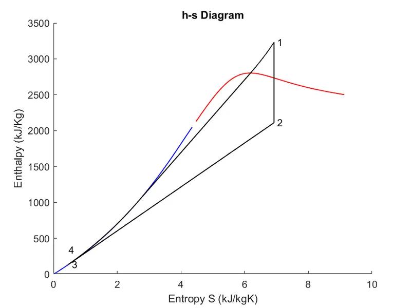
- Then, plot the corresponding T-s and h-s plots for the given set of inputs.
DISCRIPTION
Rankine Cycle
In general, the Rankine cycle is an idealized thermodynamic cycle of a constant pressure heat engine that converts part of heat into mechanical work. In this cycle, the heat is supplied externally to a closed loop, which usually uses water (in a liquid and vapor phase) as the working fluid. In contrast to the Brayton Cycle, the working fluid in the Rankine cycle undergo the phase change from a liquid to vapor phase and vice versa.
From a thermodynamics point of view, the performance of steam turbines can be derived from the theory of the Rankine cycle.
In 1859, a Scottish engineer, William John Macquorn Rankine, advanced the study of heat engines by publishing the “Manual of the Steam Engine and Other Prime Movers”. Rankine developed a complete theory of the steam engine and indeed of all heat engines. Together with Rudolf Clausius and William Thomson (Lord Kelvin), he contributed to thermodynamics, particularly focusing on the first of the three thermodynamic laws.
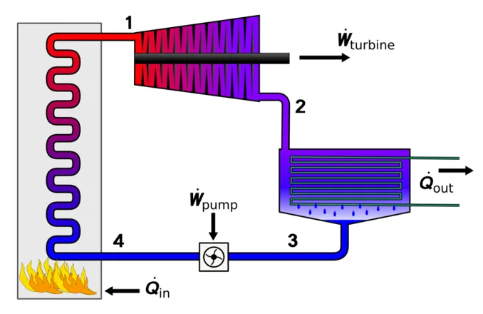
Process of Rankine cycle
In an ideal Rankine cycle, the system executing the cycle undergoes a series of four processes: two isentropic (reversible adiabatic) processes alternated with two isobaric processes:
- Isentropic expansion (expansion in a steam turbine) – Steam from the boiler expands adiabatically from state 1 to state 2 in a steam turbine to produce work and then is discharged to the condenser (partially condensed). The steam works on the surroundings (blades of the turbine) and loses an amount of enthalpy equal to the work that leaves the system. The work done by the turbine is given by WT = H1 – H2. the entropy remains unchanged.
- Isobaric heat rejection (in a heat exchanger) – In this phase, there is a constant-pressure process in which heat is rejected from the partially condensed steam. There is heat transfer from the vapor to cooling water flowing in a cooling circuit. The vapor condenses, and the temperature of the cooling water increases. The net heat rejected is given by Qre = H2 – H3.
- Isentropic compression (compression in centrifugal pumps) – The liquid condensate is compressed adiabatically from state 3 to state 1 by centrifugal pumps (usually by condensate pumps and then by feedwater pumps). The liquid condensate is pumped from the condenser into the higher-pressure boiler. In this process, the surroundings work on the fluid, increasing its enthalpy (h = u+pv) and compressing it (increasing its pressure). On the other hand, the entropy remains unchanged. The work required for the compressor is given by WP = H4 – H3.
- Isobaric heat addition (in a heat exchanger – boiler) – In this phase (between state 4 and state 1), the cycle completes by a constant-pressure heat transfer to the liquid condensate from an external source since the chamber is open to flow in and out. The feedwater (secondary circuit) is heated to the boiling point (4 → 1a) of that fluid and then evaporated in the boiler (1a → 1). The net heat added is given by Qadd = H1 – H4
During a Rankine cycle, the pumps work is done on the fluid between states 3 and 4 (isentropic compression). The fluid does work in the turbine between stages 1 and 2 (isentropic expansion). The difference between the work done by the fluid and the work done on the fluid is the network produced by the cycle, and it corresponds to the area enclosed by the cycle curve (in the pV diagram). The working fluid in a Rankine cycle follows a closed loop and is reused constantly. Wnet = WT-WP
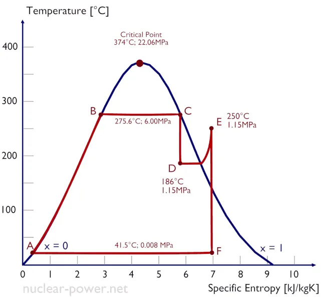
Thermal efficiency
In general, the thermal efficiency, ηth, of any heat engine is defined as the ratio of the net work it does, Wnet, to the heat input at the high temperature, Qin.
`eta_"th"=W_"net"/Q_"in"`
Specific steam consumption (SSC): It is the amount of steam required to produce unit work.
`S.S.C.=3600/(W_"net"`
Work ratio (rw): It is the ratio of the net work to turbine work.
`r_w=W_"net"/W_t`
Back work ratio (rbw): It is the ratio of the pump work to the turbine work.
`r_"bw"=W_p/W_t`
Now write a Matlab code for rankine cycle Simulator
Required Inputs
Turbine Inlet temperature = 400° C
Turbine Inlet Pressure = 30 bars
Turbine Outlet Pressure = 0.05 bars = Condenser Inlet Pressure
Xsteam libaray of Matlab
Procedure to write code
- First Display the title 'Rankine cycle Simulator' by using fprintf command.
- Display all Rankine cycle process in the command window by using fprintf command.
- and then display required inputs of pressure and temperature at turbine inlet and pressure at turbine outlet.
- Now, using Xsteam function and thermodynamic properties find the pressure, Temperature, Entropy and enthalpy at every state points.
- After that calculating net work done, efficiency, Specific steam consumption and back work ratio of the Rankine cycle.
- Now find the Entropy and Enthalpy at Saturated liquid and vapour curve with respect to Temperature range from 1 to 375 (i.e. Critical temperature of water) degree C with the help of XSteam function.
- Now plotting the T-s and h-s graph of the Rankine cycle at each state with title, axis and text labelling.
- Now Display all state point and Efficiency, Net work, Back Work Ratio, Turbine and Pump Work in command window with help of fprintf command.
The Code for rankine cycle Simulator are
clear all
close all
clc

fprintf(" \n          RANKINE CYCLE SIMULATOR        ");
fprintf('\n\n1-2 is Isentropic expansion in the Turbine');
fprintf('\n2-3 is Isobaric Heat Rejection at Condenser');
fprintf('\n3-4 is Isentropic compression in the Pump');
fprintf('\n4-1 is Isobaric Heat Addition in boiler\n');

p1=input('\nEnter the Pressure at the Turbine inlet (in Bar) : ');
t1=input('Enter the Tempurature at the Turbine inlet (in Degree Celsius) : ');
p2=input('Enter the Pressure at the Condenser inlet (in Bar) : ');

% Calculating the properties at all state of rankiine cycle
% s denote Entropy, h denote Enthalpy, x denote drayness fraction,
% t denote temperature, p denote pressure, v denote specific volume,
% state 1 ( at Turbine Inlet)
h1=XSteam('h_pT',p1,t1);       % Steam enthaply at turbine inlet
s1=XSteam('s_pT',p1,t1);       % Steam Entropy at turbine inlet

% state 2 ( at Turbine outlet or Condenser inlet)
s2=s1;
sf2=XSteam('sL_p',p2);         % Entropy at Saturated liquid curve
sg2=XSteam('sV_p',p2);         % Entropy at Saturated steam curve
x2=(s2-sf2)/(sg2-sf2);         % Dryness fraction of steam at condenser inlet
hf2=XSteam('hL_p',p2);         % Entropy at Saturated liquid curve
hg2=XSteam('hV_p',p2);         % Enthalpy at Saturated steam curve
h2=hf2+(x2*(hg2-hf2));         % Enthalpy at condenser inlet

% state 3 ( at Condenser outlet or Pump inlet)
p3=p2;
h3=XSteam('hL_p',p3);
s3=XSteam('sL_p',p3);
t3=XSteam('Tsat_p',p3);

% state 4 ( at Pump outlet or Boiler inlet)
p4=p1;
s4=s3;

% Calculate the work done by pump
v3=XSteam('vL_p',p3);          % calculating the specific volume at state 3
Wp=v3*(p4-p3)*100;

% Enthalpy at state 4
h4=h3+Wp;

% Calculating temperature at state 2, 3 and 4.
t2=XSteam('T_ps',p2,s2);
t2g=t3;

Cp4=XSteam('Cp_ps',p4,s4);      % calculating specific isobaric heat capacity at state 4
Cv4=XSteam('Cv_ps',p4,s4);      % calculating specific isochloric heat capacity at state 4
g=Cp4/Cv4;                      % Specific heat ratio of steam at state 4
k=(g-1)/g;
t4=t3*(p4/p3)^k;

% Calculating Enthalpy, Temperature and Entropy at state point 5 and 6.
s5=XSteam('sL_p',p1);
s6=XSteam('sV_p',p1);
h5=XSteam('hL_p',p1);
h6=XSteam('hV_p',p1);
t5=XSteam('Tsat_p',p1);
t6=t5;

% Calcuating Work Output by turbine
Wt=h1-h2;

% Calcuating Net Work Output
Wnet=Wt-Wp;

% Calcuating Heat energy generate by Boiler
Qin=h1-h4;

% Calaculating heat energy loss after turbine (
Qout=h2-h3;

% Calculating Efficicency of Cycle
Ntherm=Wnet/Qin;

% Calculating Specicfic Steam Consumption (kg/kWh)
S.S.C=3600/Wnet;

% Calculating Back Work Ratio
bwr=(h4-h3)/(h1-h2);

% Find the entropy and enthalpy at Saturation liquid and vapour curve
T=linspace(1,375,1000);         % Creating an array of temperature from 1 to 375 degree celisus
for i=1:length(T)
    sf(i)=XSteam('sL_T',T(i));  % Saturated liquid entropy
    sg(i)=XSteam('sV_T',T(i));  % Saturated vapour entropy
    hf(i)=XSteam('hL_T',T(i));  % Saturated liquid enthalpy
    hg(i)=XSteam('hV_T',T(i));  % Saturated vapour enthalpy
end

% Finding the entropy between t6 and t1
Ts=linspace(t6,t1,1000);       % create an array of temperature from t6 and t1
for j=1:length(Ts)             % calculate array of entropy at p1 and array of Ts
    ss(j)=XSteam('s_pT',p1,Ts(j));
end

% plotting T-s diagram
figure(1)
hold on
plot(sf,T,'b','LineWidth',1)       % plot saturated liquid curve
plot(sg,T,'r','LineWidth',1)       % plot saturated vapour curve

plot([s1 s2],[t1 t2],'k','LineWidth',1)  % plotting curve between state 1 and 2

if t2>t2g                                % plotting curve between state 2 and 3
    plot([s2 sg2],[t2 t2g],'k','LineWidth',1)
    plot([sg2 s3],[t2g t3],'k','LineWidth',1)
else
plot([s2 s3],[t2 t3],'k','LineWidth',1)
end

plot([s3 s4],[t3 t4],'k','LineWidth',1)   % plotting curve between state 3 and 4
plot([s4 s5],[t4 t5],'k','LineWidth',1)   % plotting curve between state 4 and 5
plot([s5 s6],[t5 t6],'k','LineWidth',1)   % plotting curve between state 5 and 6
plot(ss,Ts,'k','LineWidth',1)             % plotting curve between state 6 and 1

% Text state 1 to 4
text(s1+.1, t1,'1')
text(s2+.1, t2,'2')
text(s3-.25, t3+5,'3')
text(s4-.25, t4-5,'4')
text(s5-.2,t5+25,'5')
text(s6-.1,t6+25,'6')

% Labelling x and y axis and named Title of the plot
xlabel('Entropy S (kJ/kgK)')
ylabel('Temperature (degree C)')
title('T-s Diagram')

saveas(gcf,'Ts diagram.png')          % save the T-s plot

% Finding entropy between h6 and h1
ht=linspace(h6,h1,1000);                 % create an array of enthalpy from h6 and h1
for j=1:length(ht)                       % calculate array of enttropy at p1 and array of ht
    st(j)=XSteam('s_ph',p1,ht(j));
end

% Finding entropy between h4 and h5
hk=linspace(h4,h5,1000);                 % create an array of temperature from h4 and h5
for j=1:length(hk)                       % calculate array of enthalpy at p1 and array of hk
    sk(j)=XSteam('s_ph',p1,hk(j));
end

figure(2)
% plotting h-s diagram
hold on
% plotting saturated liquid and vapour curve
plot(sf,hf,'b','LineWidth',1);
plot(sg,hg,'r','LineWidth',1);
% Plotting Rankine cycle curve at state 1 to 4
plot([s1 s2],[h1 h2],'k','LineWidth',1);
plot([s2 s3],[h2 h3],'k','LineWidth',1);
plot([s3 s4],[h3 h4],'k','LineWidth',1);
plot([s5 s6],[h5 h6],'k','LineWidth',1);
plot(sk,hk,'k','LineWidth',1);
plot(st,ht,'k','LineWidth',1);
% Text state 1 to 4
text(s1+.1, h1,'1');
text(s2+.1, h2,'2');
text(s3+.1, h3,'3');
text(s4, h4+200,'4');
% Labelling x and y axis and named Title of the plot
xlabel('Entropy S (kJ/kgK)');
ylabel('Enthalpy (kJ/Kg)');
title('h-s Diagram')

saveas(gcf,'hs diagram.png')          % save the h-s plot

% Display thermodynamic properties at all states
fprintf('\n %30s \n\n','RESULTS');
fprintf('%-41s %-50s \n', 'At State Point1', 'At State point 2')
fprintf('%s %6.2f %s %30s %6.2f %s \n','P1 is',p1,'bar','P2 is',p2,'bar')
fprintf('%s %6.2f %s %28s %6.2f %s \n','T1 is',t1,'Deg C','T2 is',t2,'Deg C')
fprintf('%s %6.2f %s %27s %6.2f %s \n','H1 is',h1,'kJ/kg','H2 is',h2,'kJ/kg')
fprintf('%s %6.2f %s %27s %6.2f %s \n\n','S1 is',s1,'kJ/kgK','S2 is',s2,'kJ/kgK')

fprintf('%-41s %-50s \n', 'At State Point3', 'At State point 4')
fprintf('%s %6.2f %s %30s %6.2f %s \n','P3 is',p3,'bar','P4 is',p4,'bar')
fprintf('%s %6.2f %s %28s %6.2f %s \n','T3 is',t3,'Deg C','T4 is',t4,'Deg C')
fprintf('%s %6.2f %s %28s %6.2f %s \n','H3 is',h3,'kJ/kg','H4 is',h4,'kJ/kg')
fprintf('%s %6.2f %s %27s %6.2f %s \n\n','S3 is',s3,'kJ/kgK','S4 is',s4,'kJ/kgK')

fprintf('X2 is :%.2f \n',x2);
fprintf('Wt is :%.2f KJ/kg\n',Wt);
fprintf('Wp is :%.2f KJ/kg\n',Wp);
fprintf('Wnet is :%.2f KJ/kg\n',Wnet);
fprintf('Ntherm is :%.2f Percent\n',100*Ntherm);
fprintf('S.S.C is :%.2f kg/kWh\n', S.S.C);
fprintf('bwr is :%.2f Percent\n',100*bwr);
OUTPUTS
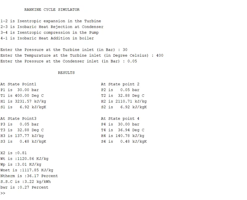
Net work ouput is 1117.85 kJ/kg
Back work ratio is 0.27%
Command window Output
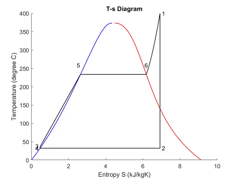
Rankine cycle T-s graph
Rankine cycle h-s graph
CONCLUSION
With the help of XSteam function and inputs, the Rankine cycle Simulator calculate thermodynamic propeties at all state points and plot T-s and h-s graph and display the output in command window.