Project 2 - Rankine cycle Simulator

AIM: To create a Rankine Cycle using the MATLAB.

OBJECTIVE
1. To calculate the state points of the Rankine Cycle based on user inputs.
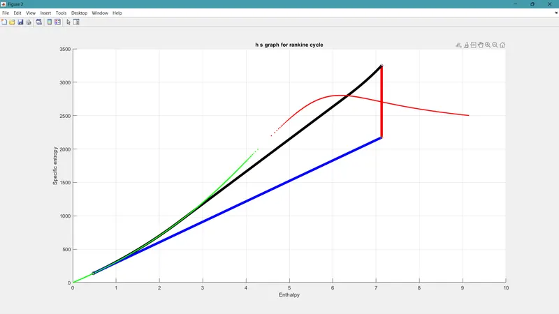
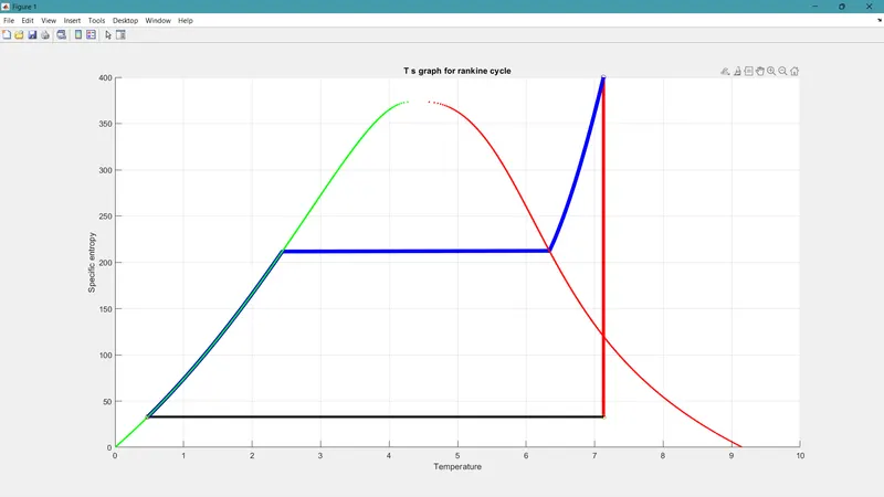
2. To plot the T-s and h-s plots for the given set of inputs.

THEORY:
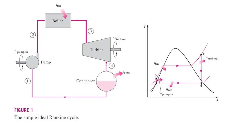
RANKINE CYCLE: THE IDEAL CYCLE FOR VAPOR POWER CYCLES
The Rankine cycle, which is the ideal cycle for vapor power plants. it has four process:

1-2 Isentropic compression in a pump
2-3 Constant-pressure heat addition in a boiler
3-4 Isentropic expansion in a turbine
4-1 Constant-pressure heat rejection in a condenser

code :

clear all
close all
clc

%description about the process
disp( 'RANKINE CYCLE' );
disp('1-2 is Isentropic Expansion in the turbine');
disp( '2-3 is constant pressure heat removal in the condenser');
disp('3-2 is Isentroplc compression in the pump');
disp('4-1 is Constant pressure heat addition in the boiler');

%input parameters
p1 = input('nValue of pressure at turbine inlet, p1(in bar) = ');
t1 = input( 'nvalue of temperature at turbine inlet, T1(in degree.C) = ');
p2 = input('nValue of temperature at condenser inlet, p2(1n bar) = ') ;

%state one points
h1 = XSteam('h_pT', p1, t1);
s1 = XSteam('s_pT', p1, t1);
v1 = XSteam('v_pT', p1, t1);

%state two points
s2=s1;
h2=XSteam('h_ps',p2,s2);
t2=XSteam('T_ps',p2,s2);
v2=XSteam('v_ps',p2,s2);

%state three points
p3 = p2;
t3 = XSteam('Tsat_p',p3)
h3 = XSteam('hL_p',p3)
s3 = XSteam('sL_p',p3)
v3 = XSteam('vL_P',p3)

%state four points
s4=s3;
p4=p1;
h4=XSteam('h_ps', p4,s4);
t4=XSteam('T_ps', p4,s4);
v4=XSteam('v_ps', p4,s4);

%plotting the graph for T vs S
figure(1)
hold on
plot([s1 s2],[t1 t2],'color','r','lineWidth',4);
plot([s2 s3], [t2 t3], 'color','k','linewidth',3);
plot([s3 s4], [t3 t4],'color', 'b','linewidth',2);
hold on
%loop for change in 4 to 1 in the t and v graph.
Temp_range = linspace(t4,t1,500);
for i=1:length(Temp_range)
    entropy_range(i) = XSteam('s_pT',p1,Temp_range(i));
    enthalpy_range_2_to_3(i) = XSteam('h_ps',p1,entropy_range(i));
    enthalpy_range_4_to_1(i) = XSteam('h_ps',p2,entropy_range(i));
end
plot(entropy_range,Temp_range,'Color','b','linewidth',5);

%plotting for the h vs s
figure(2)
hold on
plot([s1 s2],[h1 h2],'Color','r','LineWidth',5);
plot(entropy_range,enthalpy_range_2_to_3,'Color','k','linewidth',5);
plot([s3 s4], [h3 h4],'color','c','linewidth',5);
plot(entropy_range,enthalpy_range_4_to_1,'Color','b','linewidth',5);

%plotting for the change in t vs s graph
t_range = linspace(0,374.15,500);
figure(1)
hold on
for i = 1:length(t_range)
    plot(XSteam('sL_t',t_range(i)),t_range(i),'.','color','g')
    plot(XSteam('sV_t',t_range(i)),t_range(i),'.','color','r')
end

%plotting for the change in h vs s graph
figure(2)
hold on
for i = 1:length(t_range)
    plot(XSteam('sL_t',t_range(i)),XSteam('hL_t',t_range(i)),'.','color','g')
    plot(XSteam('sV_t',t_range(i)),XSteam('hV_t',t_range(i)),'.','color','r')
end

%plotting
figure(1)
hold on
plot(s1,t1,'o')
plot(s2,t2,'o')
plot(s3,t3,'o')
plot(s4,t4,'o')
xlabel('Temperature')
ylabel('Specific entropy')
title('T s graph for rankine cycle')
grid on

%plotting
figure(2)
hold on
plot(s1,h1,'o')
plot(s2,h2,'o')
plot(s3,h3,'ko')
plot(s4,h4,'ko')
xlabel('Enthalpy')
ylabel('Specific entropy')
title('h s graph for rankine cycle')
grid on

%calculating work and effieciency of the turbine and pump
boiler_heat = h1-h4;
pump_work = h4-h3;
heat_out_of_condensor = h2-h3;
turbine_work = h1-h2;
net_work = turbine_work-pump_work;
efficiency_of_rankine_cycle = net_work/boiler_heat;
specific_steam_consumption = 3600/(turbine_work-pump_work);
Back_work_ratio = turbine_work/pump_work;

clc
%printing results 
fprintf('T1= %.5f in [C] \n',t1);
fprintf('T2= %.5f in [C] \n',t2);
fprintf('T3= %.5f in [C] \n',t3);
fprintf('T4= %.5f in [C] \n',t4);

fprintf('P1= %.5f in [BAR] \n',p1);
fprintf('P2= %.5f in [BAR] \n',p2);
fprintf('P3= %.5f in [BAR] \n',p3);
fprintf('P4= %.5f in [BAR] \n',p4);

fprintf('S1= %.5f in [BAR] \n',s1);
fprintf('S2= %.5f in [BAR] \n',s2);
fprintf('S4= %.5f in [BAR] \n',s3);

fprintf('H1= %.5f in [BAR] \n',h1);
fprintf('H2= %.5f in [BAR] \n',h2);
fprintf('H3= %.5f in [BAR] \n',h3);
fprintf('H4= %.5f in [BAR] \n',h4);

fprintf('V1= %.5f in [BAR] \n',v1);
fprintf('V2= %.5f in [BAR] \n',v2);
fprintf('V3= %.5f in [BAR] \n',v3);
fprintf('V4= %.5f in [BAR] \n',v4);

    
boiler_heat = h1-h4
pump_work = h4-h3
heat_out_of_condensor = h2-h3
turbine_work = h1-h2
net_work = turbine_work-pump_work
efficiency_of_rankine_cycle = net_work/boiler_heat
specific_steam_consumption = 3600/(turbine_work-pump_work)
Back_work_ratio = turbine_work/pump_work

1.The input parameters are given by the user as t1 and p1 and p2 or p3

2.Then the remaining state points are calculated using the xsteam tables from the mathlab

3.First the first point state variables are calculated by the p1 and t1 values

4.second we calculate the state 2 values by p2 and s2 where s2=s1

5.The third point state variables are calculated by saturated liquid vapour point from p3

6.The fourth point are calcualted by the s and p values.

7.The for loop are used for the variationjs in the graphs for t s and h s graphs.

graphs :

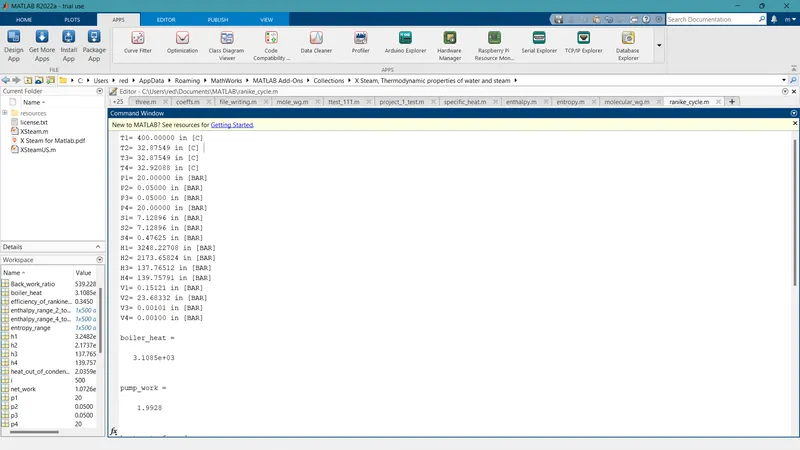
outputs:

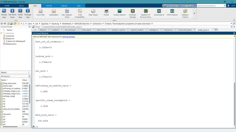
boiler_heat =

3.1085e+03

pump_work =

1.9928

heat_out_of_condensor =

2.0359e+03

turbine_work =

1.0746e+03

net_work =

1.0726e+03

efficiency_of_rankine_cycle =

0.3450

specific_steam_consumption =

3.3564

Back_work_ratio =

539.2284

boiler_heat =3.1085e+03

pump_work =1.9928

heat_out_of_condensor =2.0359e+03

turbine_work =1.0746e+03

net_work =1.0726e+03

efficiency_of_rankine_cycle =0.3450

specific_steam_consumption =3.3564

Back_work_ratio =539.2284

Results :

The ranike cycle simulation is completed by using the mathlab.