Project 1 - Parsing NASA thermodynamic data

Aim : To extarct the data from a data file and plot the properties using mathlab.

Objectives :
1. To extract the 14 coefficients and calculate the specific heat, entropy and enthalpy for all
species in the data file.
2. To calculate the molecular weight of each species.
3. To plot Specific heat, Enthalpy and Entropy with local temperature range from low temperature
to high temperature for each species.

code :

clear all
close all
clc

%data file reading
file_data = fopen('THERMO.dat','r');

%header file
header = fgetl(file_data);

%global temp
temp_data = fgetl(file_data);

global_temp = strsplit(temp_data ,' ');
global_low_temp = str2num(global_temp{2});
global_mid_temp = str2num(global_temp{3});
global_high_temp = str2num(global_temp{4});

%for loop to read three lines
for i=1:3
    fgetl(file_data)
end


%for loop for reading species data
for i = 1:53
    Line_1 = fgetl(file_data);
    line_desc = strsplit(Line_1);
    species_name = line_desc{1};
    local_low_temp = str2double(line_desc{6});
    local_mid_temp = str2double(line_desc{8});
    local_high_temp = str2double(line_desc{7});

    temp = linspace(local_low_temp,local_high_temp,500);
    
    Line_2 = fgetl(file_data);
    ee = strfind(Line_2 , 'E');

    Line_3 = fgetl(file_data);
    eee = strfind(Line_3 , 'E');

    Line_4 = fgetl(file_data);
    eeee = strfind(Line_4 , 'E');

     %high temp coeff's
    a1 = str2double(Line_2(1:ee(1)+3));
    a2 = str2double(Line_2(ee(1)+4:ee(2)+3));
    a3 = str2double(Line_2(ee(2)+4:ee(3)+3));
    a4 = str2double(Line_2(ee(3)+4:ee(4)+3));
    a5 = str2double(Line_2(ee(4)+4:ee(5)+3));
    a6 = str2double(Line_3(1:eee(1)+3));
    a7 = str2double(Line_3(eee(1)+4:eee(2)+3));

    %low temp coeff's

    a8 = str2double(Line_3(eee(2)+4:eee(3)+3));
    a9 = str2double(Line_3(eee(3)+4:eee(4)+3));
    a10 = str2double(Line_3(eee(4)+4:eee(5)+3));
    a11 = str2double(Line_4(1:eeee(1)+3));
    a12 = str2double(Line_4(eeee(1)+4:eeee(2)+3));
    a13 = str2double(Line_4(eeee(2)+4:eeee(3)+3));
    a14 = str2double(Line_4(eeee(3)+4:eeee(4)+3));
    
    R = 8.314;
    c_p = specific_heat(a1,a2,a3,a4,a5,a6,a7,a8,a9,a10,a11,a12,a13,a14,R,temp,local_mid_temp);
    h = enthalpy(a1,a2,a3,a4,a5,a6,a8,a9,a10,a11,a12,a13,R,temp,local_mid_temp);
    s = entropy(a1,a2,a3,a4,a5,a7,a8,a9,a10,a11,a12,a14,R,temp,local_mid_temp);
    Mw = molecular_wg(species_name)

     %plotting graphs
    figure(1)
    plot(temp,h,'linewidth',2,'Color','r');
    title('temp vs enthalpy',species_name);
    xlabel('temp')
    ylabel('Enthalpy')
    grid on

    figure(2)
    plot(temp,s,'linewidth',2,'Color','r');
    title('temp vs entropy',species_name);
    xlabel('temp')
    ylabel('Entropy')
    grid on

    figure(3)
    plot(temp,c_p,'linewidth',2,'Color','r');
    title('temp vs specific heat',species_name);
    xlabel('temp')
    ylabel('specific heat')
    grid on
     %saving data
    mkdir(species_name);
    cd(species_name);

    saveas(1,'enthalpy.jpg')
    saveas(2,'entropy.jpg')
    saveas(3,'specific_heat.jpg')

    cd  ..


     %displaying ouput to command window
    disp(['molecular weight of ',species_name]);
    disp(Mw);

end


fclose(file_data)

Code Explanation :

1.To read the data from the Nasa file, we can use the fopen command and we can use the fgetl command is used
to get the next line.
2.First the header information.
3.The next line we have global temperatures values we are read by using the strsplit command, then we used Str2num is
used to convert strings to numbers.
4.Next the three lines are read by using the for loop
5.The local temperatures values are read by using the for loop and we have 53 species in the given data.
6.we used the strsplit command to split the data and strfind to find the value of E and by that we read the data.
7.we plotted the c_p,h,s from the function we denoted.
8.The mw are stored in the folder.

Entropy:

function [s] = entropy(a1,a2,a3,a4,a5,a7,a8,a9,a10,a11,a12,a14,R,temp,local_mid_temp)
if temp <= local_mid_temp
    s = R.*(a8.log(temp) + (a9.*temp)+ (a10.*((temp).^2)./2)+(a11.*((temp).^3)./3)+(a12.*((temp).^4)./4)+a14);
else
    s = R.*(a1.*log(temp) + (a2.*temp)+ (a3.*((temp).^2)./2)+(a4.*((temp).^3)./3)+(a5.*((temp).^4)./4)+a7);
end
end

Enthalpy:

function [h] = enthalpy(a1,a2,a3,a4,a5,a6,a8,a9,a10,a11,a12,a13,R,temp,local_mid_temp)
if temp <= local_mid_temp
    h = R*temp.*(a8 + (a9.*temp./2)+ (a10.*((temp).^2)./3)+(a11.*((temp).^3)./4)+(a12.*((temp).^4)./5)+a13.*temp);
else
    h = R*temp.*(a1 + (a2.*temp./2)+ (a3.*((temp).^2)./3)+(a4.*((temp).^3)./4)+(a5.*((temp).^4)./5)+a6.*temp);
end
end

Specific heat :

function [c_p] = specific_heat(a1,a2,a3,a4,a5,a6,a7,a8,a9,a10,a11,a12,a13,a14,R,temp,local_mid_temp)
if temp <= local_mid_temp
    c_p = (a8 + (a9.*temp)+ (a10.*((temp)).^2)+(a11.*((temp).^3))+(a12.*((temp).^4)));
else
    c_p = (a1 + (a2.*temp)+ (a3.*((temp)).^2)+(a4.*((temp).^3))+(a5.*((temp).^4)));
end
end

Molecular weight :

function [Mw] = molecular_wg(species_name)

elements = ['H','C','N','O','R'];
atomic_weight = [1, 12, 14, 16, 40];

Mw = 0;
for i = 1:length(species_name)
    for j=1:length(elements)
        if strcmpi(species_name(i),elements(j))
            Mw = Mw + atomic_weight(j);
            position = j;
        end
    end
n = str2double(species_name(i));
if n>1
        Mw = Mw + (atomic_weight(position))*(n-1);
end
end
end

Graphs :

carbon

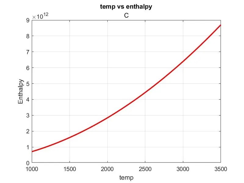
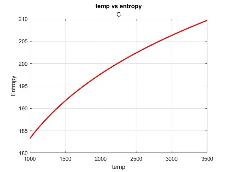
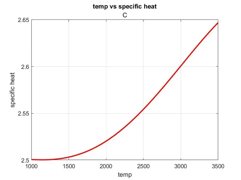
oxygen

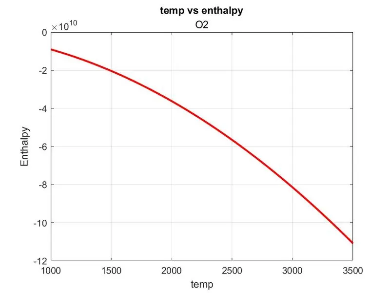
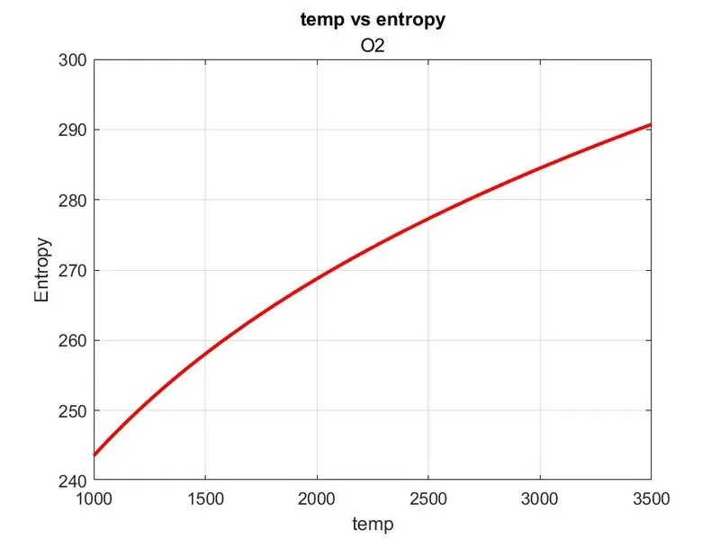
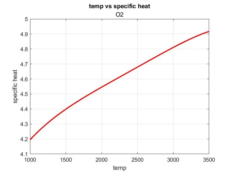
molecualr weights outputs data

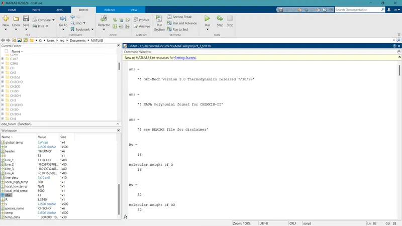
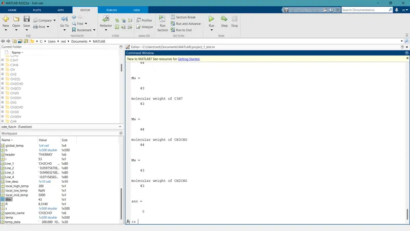
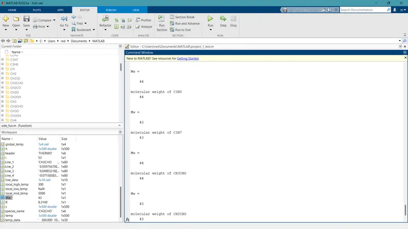
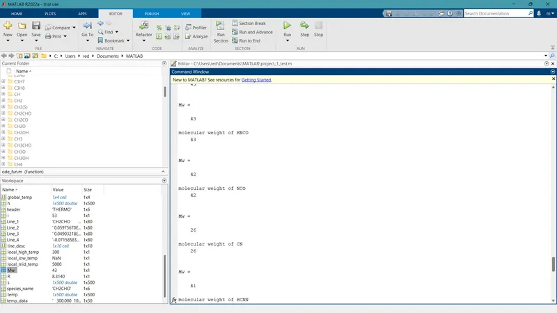
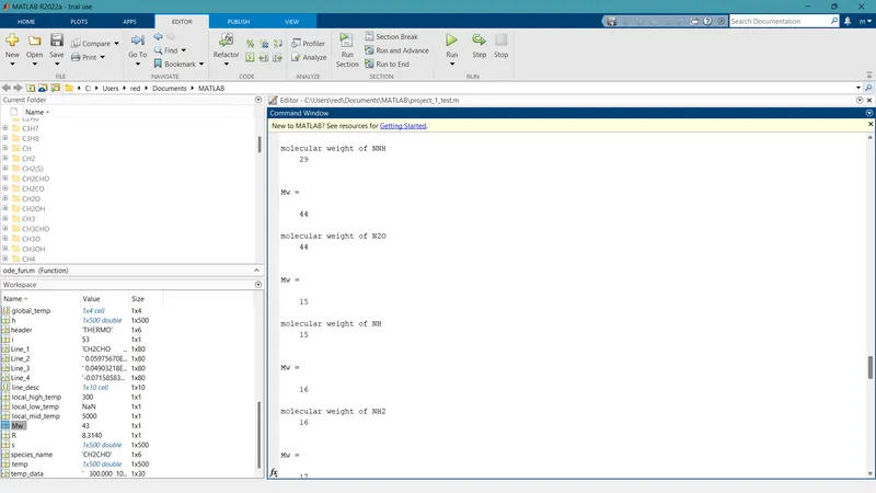
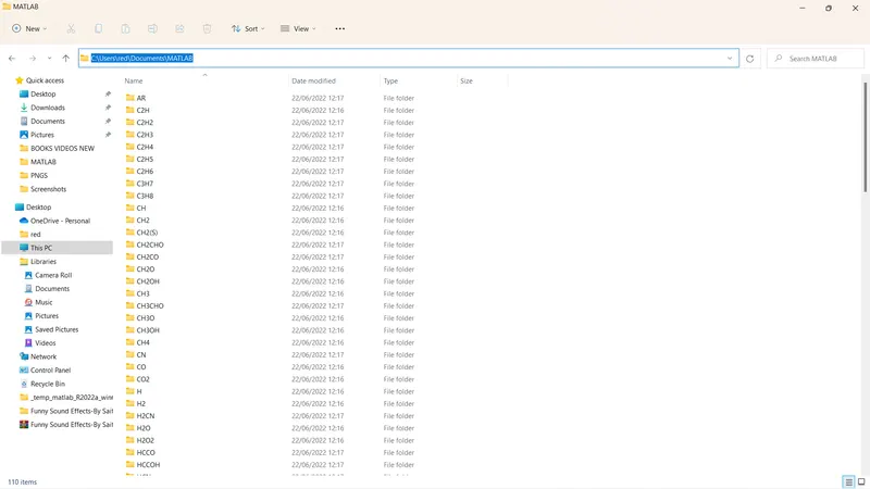
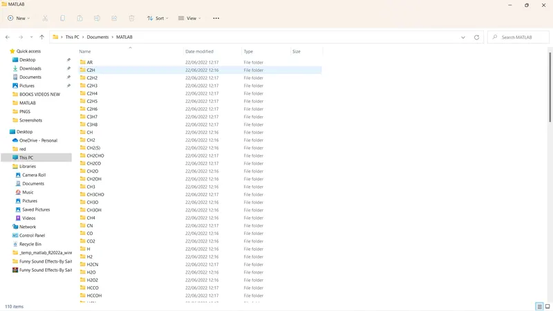
Results : The data from the file is read and the required garphs are plotted using the mathlab

references :

https://in.mathworks.com/help/matlab/ref/str2num.html?searchHighlight=str2num&s_tid=srchtitle_str2num_1

https://skill-lync.com/student-projects/project-1-parsing-nasa-thermodynamic-data-455