Project 2 - Rankine cycle Simulator

Aim: To create Rankine Cycle Simulator.

Objective:

• To calculate the state points of the Rankine cycle based on user inputs.
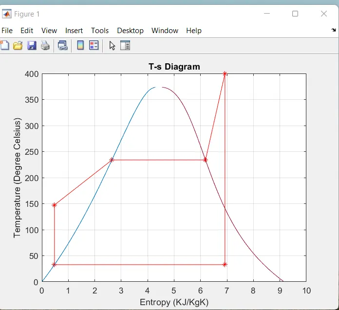
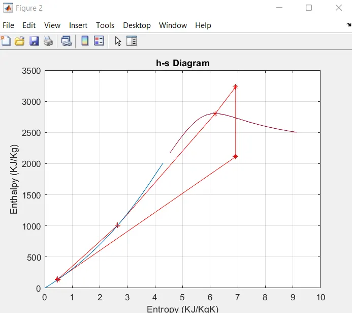
• To plot T-S and h-S plots.
• To calculate Net work output.
• To calculate Back work ratio.

Concept:

Rankine Cycle:A Rankine cycle power system is a heat engine converting thermal energy into work.It comprises four main components: a boiler (sometimes called evaporator), a turbine, a condenser and a pump . The working fluid in a low-pressure slightly subcooled liquid state is brought to high pressure by the pump. The pump consumes power. The high-pressure liquid enters the boiler, where it is heated-up, vaporized and potentially heated again to leave the boiler in superheated vapor state. Thermal power must be supplied to the boiler by an external heat source. At the outlet of the boiler, the high-pressure vapor enters the turbine where it is expanded down to the low pressure. The turbine delivers mechanical power. As a function of the nature of the working fluid and turbine inlet state, the fluid at the end of the expansion can be in superheated vapor state or in two-phase state. At the outlet of the turbine, the fluid enters the condenser where it is condensed to liquid state and, then, slightly subcooled. Thermal power rejected at the condenser is dumped into a heat sink. The low-pressure subcooled liquid enters the pump again.

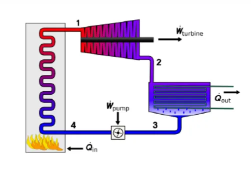
It consists of four process.

1.Process 1-2 : Isentropic Expansion in Turbine

Dry saturated vapour expand in turbine,generate power.The shaft is connected to generator,this results in production of electricity means conversion of Mechanical energy to Electric energy.

2.Process 2-3: Constant pressure Heat rejection in condenser

The expanded vapour passed through condenser,where it gets condensed and converted into liquid again.This liquid goes into the boiler.

3.process 3-4:Isentropic compression by pump:

water comes into the pump in saturated liquid state and it gets compressed isentropically in the pump to the boiler pressure.

4.process 4-1:Constant pressure Heat addition :

water changes into high pressure steam where pressure will be constant.

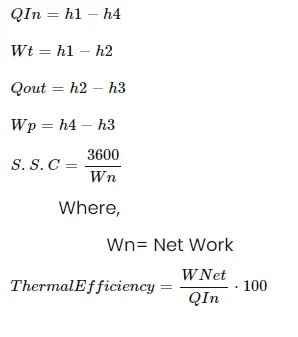
Govering Equation:

Input parameters :

Turbine inlet temperature(t1)=400°C

Turbine inlet pressure=30bars

Turbine outlet pressure =0.05 bar = condenser inlet pressure

Main programme:

clear all
close all
clc

disp('                RANKINE CYCLE SIMULATOR  ');
disp('  ');
disp(' 1-2 Isentropic Expansion in the Turbine');
disp(' 2-3 Constant Pressure Heat Rejection in the condenser');
disp(' 3-4 Isentropic Compression in the Pump');
disp(' 4-1 Constant pressure Heat Addition in the Boiler');

%Getting inputs
P1=input('Enter the Pressure at the Turbine Inlet (bar): ');
T1=input('Enter the Temperature at the Turbine Inlet (Degree Celsius): ');
P2=input('Enter the Pressure at the Condenser(bar): ');

%Solving the Rankine Cycle

%Creating the high pressure line
Tsat1=XSteam('Tsat_P',P1);
Cpv1=XSteam('CpV_p',P1);
Cpv11=XSteam('CpL_p',P1);
Cpv4=XSteam('CpV_p',P1);
Cp14=XSteam('CpL_p',P1);

%At Point 1'
hg1=XSteam('hV_p',P1);
sg1=XSteam('SV_p',P1);

%At Point 4'
hf1=XSteam('hL_p',P1);
sf1=XSteam('SL_p',P1);

%Creating the low pressure line
Tsat2=XSteam('Tsat_p',P2);
Cpv2=XSteam('CpV_p',P2);
Cp12=XSteam('CpL_p',P2);
Cpv3=XSteam('CpV_p',P2);
Cp13=XSteam('CpL_p',P2);

%At point 2'
hg2=XSteam('hV_p',P2);
sg2=XSteam('SV_p',P2);

%At point 3
hf2=XSteam('hL_p',P2);
sf2=XSteam('SL_p',P2);

%Calculating the State variables

% At State point 1
h1=XSteam('h_pT',P1,T1);
s1=XSteam('S_pT',P1,T1);

% At State Point 2
s2=s1;
if (s2<=sg2)
        x2=(s2-sf2)/(sg2-sf2);
else
    x2=1;
end

if (x2<1)
    T2=Tsat2;
    h2=hf2+x2*(hg2-hf2);
else
    % s= sg2+Cpv2*ln(T2+273/Tsat+273)
    T2=((Tsat2+273)*exp((s2-sg2)/Cpv2))-273;
    h2=hg2+Cpv2*(T2-Tsat2);
end

% At State  Point 3(No Subcooling Condition)
P3=P2;
T3=Tsat2;
h3=hf2;
s3=sf2;
V3=XSteam('vL_p',P3);

% At state Point 4
P4=P1;
s4=s3;
Wp=(P4-P3)*V3*100;
%Wp= h4-h3;
h4=h3+Wp;
%s4=sf1+Cp14*ln(T4/Tsat)
T4=(Tsat1*exp((s4-sf1)/Cp14));
h41=XSteam('hL_p',P4);
s41=XSteam('sL_p',P4);
h42=XSteam('hV_p',P4);
s42=XSteam('sV_p',P4);
T41=XSteam('T_hs',h41,s41);
T42=XSteam('T_hs',h42,s42);
Wt=h1-h2;
Wnet=Wt-Wp;
Qin=h1-h4;
Qout=h2-h3;
Ntherm=Wnet/Qin;
SSC=3600/Wt;

%Creating Saturation Curve
T=linspace(1,T1,1000);
for i=1:length(T)
    hl(i)=XSteam('hL_T',T(i));
    hv(i)=XSteam('hV_T',T(i));
    sl(i)=XSteam('sL_T',T(i));
    sv(i)=XSteam('sV_T',T(i));
end

%Getting the desired output
fprintf('    RESULTS \n')
fprintf('\n  At State Point1: \n')
fprintf('P1 = %f bar \n',P1)
fprintf('T1 = %f Degreee Celsius \n',T1)
fprintf('h1 = %f KJ/Kg \n',h1)
fprintf('s1 = %f  KJ/KgK \n',s1)

fprintf('\n  At State Point2: \n')
fprintf('P2 = %f bar \n',P2)
fprintf('T2 = %f Degreee Celsius \n',T2)
fprintf('h2 = %f KJ/Kg \n',h2)
fprintf('s2 = %f  KJ/KgK \n',s2)


fprintf('\n  At State Point3: \n')
fprintf('P3 = %f bar \n',P3)
fprintf('T3 = %f Degreee Celsius \n',T3)
fprintf('h3 = %f KJ/Kg \n',h3)
fprintf('s3 = %f  KJ/KgK \n',s3)

fprintf('\n  At State Point4: \n')
fprintf('P4 = %f bar \n',P4)
fprintf('T4 = %f Degreee Celsius \n',T4)
fprintf('h4 = %f KJ/Kg \n',h4)
fprintf('s4 = %f  KJ/KgK \n',s4)

fprintf('\n Other Parameters: \n ')
fprintf('Wt = %f KJ/Kg \n',Wt)
fprintf('Wp = %f KJ/Kg \n',Wp)
fprintf('Wnet = %f KJ/Kg \n',Wnet)
fprintf('Ntherm= %f   percentage \n',Ntherm)
fprintf('S.S.C= %f Kg/KWhr \n',SSC)


%plotting Graphs

% T-s Diagram
figure(1)

plot([s1 s2 ],[T1 T2 ],[s2 s3],[T2 T3],[s3 s4],[T3 T4],[s4 s41],[T4 T41],[s41 s42],[T41 T42],[s42 s1],[T42 T1],'Marker','*','Color','r')
hold on
plot(sv,T)
plot(sl,T)
xlabel('Entropy (KJ/KgK)')
ylabel('Temperature (Degree Celsius)')
title('T-s Diagram')
grid on

% h-s Diagram
figure(2)

plot([s1 s2 ],[h1 h2 ],[s2 s3],[h2 h3],[s3 s4],[h3 h4],[s4 s41],[h4 h41],[s41 s42],[h41 h42],[s42 s1],[h42 h1],'Marker','*','Color','r')
hold on
plot(sv,hv)
plot(sl,hl)

xlabel('Entropy (KJ/KgK)')
ylabel('Enthalpy (KJ/Kg)')
title('h-s Diagram')
grid on
hold off

Explanation:

1.The user Inputs are taken.

2.Properties such as Temperature T, Entropy S,Enthalpy h,Pressure P is calculated by using some relations and XStream library.

3.Dryness fraction is calculated here.T2 and h2 also claculated by using dryness fraction

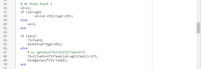
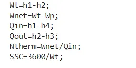
4.Output parameters are calculated by their respective formulas

5.For creating the saturation curve we have taken 1000 temperature values between 1 to T1.

6.T-s and h-s graph is plotted.

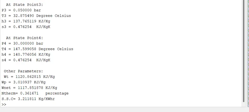
7.By using fprintf command the output results are showned in the command window.

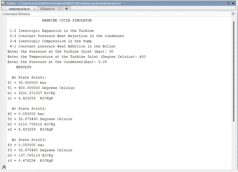
Output:

Diagrams: