Project 2 - Rankine cycle Simulator
Aim:
To create a Rankine Cycle Simulator using OCTAVE/MATLAB.
Objective:
- Create a Rankine Cycle Simulator using OCTAVE/MATLAB.
- Your code should calculate the state points of the Rankine Cycle (any type of your choice) based on user inputs.
- Then, plot the corresponding T-s and h-s plots for the given set of inputs. Title and axes labels are a must, while legends could be used if necessary.
- The presentation of your code will be taken into consideration while grading. Labelling sections of your code using comments is appreciated.
- Attach a report explaining the working of a rankine cycle simulator and also the research done by you.
Rankine Cycle:
The Rankine cycle is an idealized thermodynamic cycle describing the process by which certain heat engines, such as steam turbines or reciprocating steam engines, allow mechanical work to be extracted from a fluid as it moves between a heat source and heat sink. Heat energy is supplied to the system via a boiler where the working fluid (typically water) is converted to a high pressure gaseous state (steam) in order to turn a turbine. After passing over the turbine the fluid is allowed to condense back into a liquid state as waste heat energy is rejected before being returned to boiler, completing the cycle. Friction losses throughout the system are often neglected for the purpose of simplifying calculations as such losses are usually much less significant than thermodynamic losses, especially in larger systems.
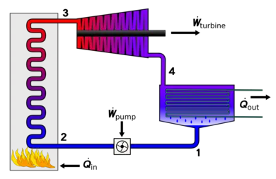
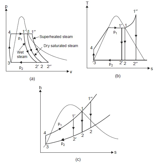
Process 1-2: Reversible adiabatic expansion in the turbine (or steam engine).
Process 2-3: Constant-pressure transfer of heat in the condenser.
Process 3-4: Reversible adiabatic pumping process in the feed pump.
Process 4-1: Constant-pressure transfer of heat in the boiler.
Applying steady flow energy equation (S.F.E.E.) to boiler, turbine, condenser and pump:
(i) For boiler (as control volume), we get
f4 + Q1 = h1
Q1 = hl - hf4
(ii) For turbine (as control volume), we get
h1 = WT + h2, where WT = turbine work
WT = hl - h2
(iii) For condenser, we get
h2 = Q2 + hf3
Q2 = h2 - hf3
(iv) For the feed pump, we get
hf3 + WP = hf4, where WP = Pump work
WP = hf4-hf3 = v3 (p1 - p2)
Efficiency of Rankine cycle is given by
η =w/Qnet1=WT-WP/Q1
Program:
clear all
close all
clc

%information
fprintf('    RANKINE CYCLE SIMULATOR      \n')
fprintf(' 1-2 Isentropic Expansion in Turbine\n');
fprintf(' 2-3 Constant Pressure Heat Rejection in the Condenser\n');
fprintf(' 3-4 Isentropic Compression in the Pump\n');
fprintf(' 4-1 Constant Pressure Heat Addition by the Boiler\n');

%inputs
p1=input(' Enter the Pressure at the Turbine inlet (bar): ');
t1=input(' Enter the Temperature at the Turbine inlet (celsius) : ');
p2=input(' Enter the Pressure at the Condenser (bar): ');

% @ stage 1 Turbine Inlet
% p1 & t1 are given
h1=XSteam('h_pt',p1,t1);
s1=XSteam('s_pt',p1,t1);

% @ stage 2 Condenser Inlet
%p2 is given
s2=s1;
sf2=XSteam('sL_p',p2);
sg2=XSteam('sV_p',p2);
hf2=XSteam('hL_p',p2);
hg2=XSteam('hV_p',p2);
x2=(s2-sf2)/(sg2-sf2);
h2=hf2+(x2*(hg2-hf2));

% @ stage 3 Pump Inlet
p3=p2;
h3=XSteam('hL_p',p3);
s3=XSteam('sL_p',p3);
t3=XSteam('Tsat_p',p3);
t2=t3;

% @ stage 4 Boiler Inlet
p4=p1;
s4=s3;
h4=XSteam('h_ps',p4, s4);

cp4=XSteam('Cp_ps',p4, s4);
cv4=XSteam('Cv_ps',p4, s4);
lambda=cp4/cv4;
t4=t3/((p3/p4)^((lambda-1)/lambda));

t5=XSteam('Tsat_p',p1);
t6=t5;
s5=XSteam('sL_p',p1);
s6=XSteam('sV_p',p1);
h5=XSteam('hL_p',p1);
h6=XSteam('hV_p',p1);

% Turbine Work
Wt=h1-h2;

% Pump Work
Wp=h4-h3;

% Net Work (kJ/kg)
W=Wt-Wp;

% Heat in & out of the System
Q_in=h1-h4;
Q_out=h2-h3;

% Thermal Efficiency
ntherm=(W/Q_in)*100;

% Steam rate (kg/kWh)
SSC=3600/W;

% Back Work Ratio
BWR=(h1-h4)/(h2-h3);

% to plot Saturation Curve
T=linspace(1,400,500);
for i=1:length(T)
  h_l(i)=XSteam('hL_T',T(i));
  h_v(i)=XSteam('hV_T',T(i));
  s_l(i)=XSteam('sL_T',T(i));
  s_v(i)=XSteam('sV_T',T(i));
end

% plotting TS diagram
figure(1)
hold on
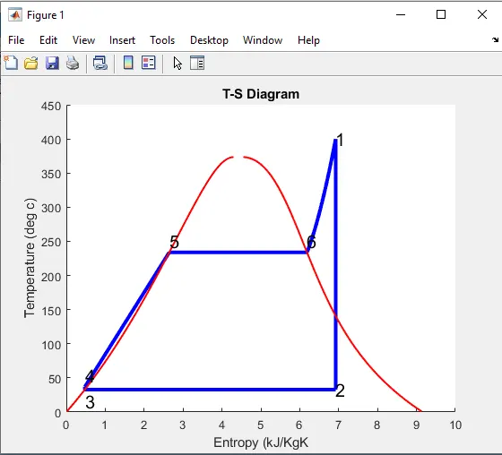
title('T-S Diagram')
plot([s1 s2],[t1 t2],'linewidth',3,'color','b')
plot([s2 s3],[t2 t3],'linewidth',3,'color','b')
plot([s3 s4],[t3 t4],'linewidth',3,'color','b')
plot([s4 s5],[t4 t5],'linewidth',3,'color','b')
plot([s5 s6],[t5 t6],'linewidth',3,'color','b')
xlabel('Entropy (kJ/KgK');
ylabel('Temperature (deg c)');
s_1=linspace(s6,s1,500);
for j=1:length(s_1)
  t_1(j)=XSteam('T_ps',p1,s_1(j));
end
plot(s_1,t_1,'linewidth',3,'color','b')
plot(s_l,T,'linewidth',1.5,'color','r')
plot(s_v,T,'linewidth',1.5,'color','r')

% Annotations
text(s1,t1,'1','fontsize',15);
text(s2,t2,'2','fontsize',15);
text(s3,t3,'3','fontsize',15,'verticalalignment','top');
text(s4,t4,'4','fontsize',15,'verticalalignment','bottom');
text(s5,t5,'5','fontsize',15,'verticalalignment','bottom');
text(s6,t6,'6','fontsize',15,'verticalalignment','bottom');

figure(2)
hold on
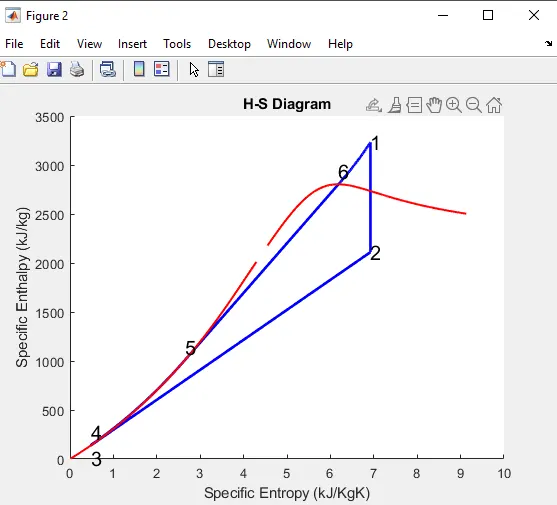
title('H-S Diagram');
plot([s1 s2],[h1 h2], 'linewidth',2,'color','b')
plot([s2 s3],[h2 h3], 'linewidth',2,'color','b')
plot([s3 s4],[h3 h4], 'linewidth',2,'color','b')

h_4=linspace(h4,h5,500);
for k=1:length(h_4)
  s_4(k)=XSteam('s_ph',p1,h_4(k));
end

h_6=linspace(h6,h1,500);
for m=1:length(h_6)
  s_6(m)=XSteam('s_ph',p1, h_6(m));
end

plot(s_4,h_4,'linewidth',2,'color','b')
plot([s5 s6],[h5 h6],'linewidth',2,'color','b')
plot(s_6,h_6, 'linewidth',2,'color','b')
xlabel('Specific Entropy (kJ/KgK)');
ylabel('Specific Enthalpy (kJ/kg)');
plot(s_l,h_l,'linewidth',1.5,'color','r')
plot(s_v,h_v,'linewidth',1.5,'color','r')

% Annotations
text(s1,h1,'1','fontsize',15);
text(s2,h2,'2','fontsize',15);
text(s3,h3,'3','fontsize',15,'verticalalignment','top');
text(s4,h4,'4','fontsize',15,'verticalalignment','bottom');
text(s5,h5,'5','fontsize',15,'verticalalignment','bottom');
text(s6,h6,'6','fontsize', 15,'verticalalignment','bottom');

% Results Window
fprintf('RESULTS \n');
fprintf('At State Point 1\n');
fprintf('P1=%f Bar\n',p1);
fprintf('T1=%f Deg Celsius\n',t1);
fprintf('H1=%f kJ/kg\n', h1);
fprintf('S1=%f kJ/kgk\n',s1);

fprintf('At State Point 2\n');
fprintf('P2=%f Bar\n',p2);
fprintf('T2=%f Deg Celsius\n',t2);
fprintf('H2=%f kJ/kg\n',h2);
fprintf('S2=%f kJ/Kgk',s2);

fprintf('At State Point 3\n');
fprintf('P3=%f Bar\n',p3);
fprintf('T3=%f Deg Celsius\n',t3);
fprintf('H3=%f kJ/kg\n',h3);
fprintf('S3=%f kJ/kgk\n',s3);

fprintf('At State Point 4\n');
fprintf('P4=%f Bar\n',p4);
fprintf('T4=%f Deg Celsius\n',t4);
fprintf('H4=%f kJ/kg\n',h4);
fprintf('S4=%f kJ/kgk\n', s4);

fprintf('Work done by Turbine is : %f kJ/kg\n', Wt);
fprintf('Work done by Pump is : %f kJ/Kg\n', Wp);
fprintf('Net Work done on the system : %f kJ/Kg\n',W);
fprintf('Specific Steam Consumption is : %f kg/KWh\n',SSC);
fprintf('The Net Thermal Efficiency of the System is : %f\n',ntherm);
fprintf('The BWR of the Rankine Cycle is found to be : %f\n', BWR);
Explanation:
The program starts with clear all,close all and clc to clear the command windoe,workspace and the plots. The printf command is used to print a series of information on the command window.
The values of p1,t1 and p2 are given as inputs whose values are to be entered in the command window on executing the program.
XSteam.m file is used to extract the data for the Rankine cycle it consist of water &steam properties.In State-1, Values for Enthalpy & Entropy are extracted as a function of Pressure & Temperature. oh_PT, S_PT, hL_p, SV_p etc.... are the default variables whose value is stored in XSteam file.
Similarly all the variables for all states are extracted using suitable format.
The equation for the rankine cycle are derived from the p-v and t-s diagrams.Pressure, Temperature, Enthalpy, Entropy forall the State Variables are Extracted as a function of dependent
variable from the XSteam File.
State 2 is an condenser inlet where the dry saturated steam is condensed into liquid.Enthalpy & Entropy for Saturated Vapour & Saturated Water are considered to Calculate the
Specific Enthalpy.
In state 3 the condensed water is feeded into the pump. It is an pressure addition process. The temperature of the water remains the same. The state 4 is a constant Pressure Heat addition, hence pressure is equal to pl, but the temperature increases on heating at Constant Pressure & Constant Volume as our Entropy remains same and hence Cp/Cv=lambda is considered to find temperature T4.Finally Work done and Heat Evolved & SSC are calculated by basic formulae.To plot the Saturation Curve, a Temerature range is defined using linspace command and for the overall length
of this Temperature values of Enthalpy and Entropy are calculated at every temperature point. The Break in the Saturation Curve seperates the Liquid Phase & Vapour Phase. Now all the necessary data is find out, Plotting is done for both T-S & H-S curves using the plot commands.
Annotations are assigned using text command. Results of the Cycle Simulation is displayed over command window using fprintf command. Back Work Ratio (BWR) is defined as the fraction of the work produced by the turbine that is consumed by the pump. BWR should range from 1 to 2 for Vapour Power Cycle like Rankine.
Output:
Command Window:
RANKINE CYCLE SIMULATOR
1-2 Isentropic Expansion in Turbine
2-3 Constant Pressure Heat Rejection in the Condenser
3-4 Isentropic Compression in the Pump
4-1 Constant Pressure Heat Addition by the Boiler
Enter the Pressure at the Turbine inlet (bar): 30
Enter the Temperature at the Turbine inlet (celsius) : 400
Enter the Pressure at the Condenser (bar): 0.05
RESULTS
At State Point 1
P1=30.000000 Bar
T1=400.000000 Deg Celsius
H1=3231.571027 kJ/kg
S1=6.923259 kJ/kgk
At State Point 2
P2=0.050000 Bar
T2=32.875490 Deg Celsius
H2=2110.708212 kJ/kg
S2=6.923259 kJ/KgkAt State Point 3
P3=0.050000 Bar
T3=32.875490 Deg Celsius
H3=137.765119 kJ/kg
S3=0.476254 kJ/kgk
At State Point 4
P4=30.000000 Bar
T4=36.935287 Deg Celsius
H4=140.762226 kJ/kg
S4=0.476254 kJ/kgk
Work done by Turbine is : 1120.862815 kJ/kg
Work done by Pump is : 2.997107 kJ/Kg
Net Work done on the system : 1117.865709 kJ/Kg
Specific Steam Consumption is : 3.220423 kg/KWh
The Net Thermal Efficiency of the System is : 36.167417
The BWR of the Rankine Cycle is found to be : 1.566598
>>
Errors:
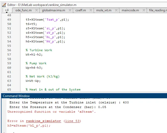
Did a typeover here in the word xStream, and then recognized it.
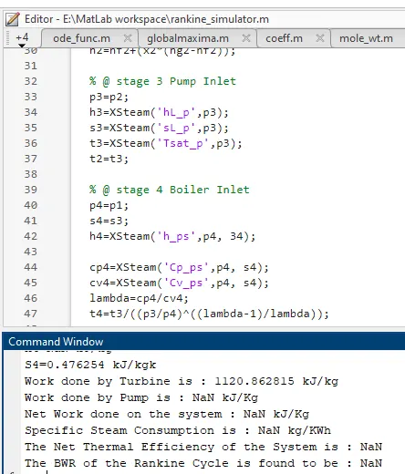
In h4 i did a typing mistake instead of s4 I have typed 34 and i got the values of work done, net work done as NaN. Later I found out and changed it.
Conclusion:
We have created a Rankine cycle simulator using MatLab and also the objective has been acheived.