Project 2 - Rankine cycle Simulator
Report on Rankine cycle Simulator
Aim:
- To create a Rankine Cycle Simulator using MATLAB.
- To calculate the Net work output, Back work ratio.
Required Inputs:
- Turbine Inlet temperature = 400° C.
- Turbine Inlet Pressure = 30 bars.
- Turbine Outlet Pressure = 0.05 bars = Condenser Inlet Pressure.
Required Output:
Software Used: MATLAB.
Code:
%code for Rankine cycle
clear all
close all
clc
%To print some data
fprintf(" Rankine cycle \n")
fprintf("1-2:Isentropic compression in the pump\n")
fprintf("2-3:Constant pressure heat addition in a boiler\n")
fprintf("3-4:Isentropic expansion in a turbine\n")
fprintf("4-1:Constant pressure heat rejection in a condenser\n")
%Obtaining the input data
p1=input('Enter turbine inlet pressure ~');
T1=input('Enter turbine inlet temprature ~');
p2=input('Enter turbine outlet pressure ~');
%Extracting data
%state1
%extracting enthalphy at state 1
h1=XSteam('h_pT',p1,T1);
%extracting entrophy at state 1
s1 = XSteam('s_pT',p1,T1);
%state2
s2=s1;
%saturated liquid entrophy
sf2=XSteam('sL_p',p2);
%saturated vapour entrophy
sg2=XSteam('sV_p',p2);
x2=(s2-sf2)/(sg2-sf2);
hf2= XSteam('hL_p',p2);
hg2=XSteam('hV_p',p2);
h2=hf2+(x2*(hg2-hf2));
%state3
p3=p2;
s3=XSteam('sL_p',p3);
h3=XSteam('hL_p',p3);
%state4
s4=s3;
p4=p1;
%workdone by the turbine
wt=h1-h2;
%workdone to run a pump
v3=XSteam('vL_p',p3);
wp=v3*(p4-p3)*100;
h4=h3+wp;
%calculating net work
w_net=wt-wp;
%heat into the system
Qin=h1-h4;
%heat out from the system
Qout=h2-h3;
%To calculate Thermal efficiency
therm_efficiency=(w_net/Qin)*100;
%calculating work ratio
work_ratio=(w_net/wt);
%calculating back work ratio
back_work_ratio=(h1-h4)/(h2-h3);
%calculating temperature at the state points
T3=XSteam('Tsat_p',p3);
T2=T3;
Cp4=XSteam('Cp_ps',p4,s4);
Cv4=XSteam('Cv_ps',p4,s4);
k=Cp4/Cv4;
T4=T3/((p3/p4)^((k-1)/k));
%calulating temp,entrophy,enthalphy
T6=XSteam('Tsat_p',p1);
s5=XSteam('sL_p',p1);
s6=XSteam('sV_p',p1);
h5=XSteam('hL_p',p1);
h6=XSteam('hV_p',p1);
T5=T6;
%plotting the saturation curve
%temprature of water is=374
T=linspace(1,375,1000);
for i=1:length(T)
sf(i)=XSteam('sL_T',T(i));
sg(i)=XSteam('sV_T',T(i));
hf(i)=XSteam('hL_T',T(i));
hg(i)=XSteam('hV_T',T(i));
end
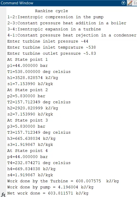
%displaying results
%state point 1
fprintf('At State point 1 \n')
fprintf('p1=%f bar\n',p1)
fprintf('T1=%f deg celsius\n',T1)
fprintf('h1=%f kJ/kg\n',h1)
fprintf('s1=%f kJ/kgk\n',s1)
fprintf('At State point 2 \n')
fprintf('p2=%f bar\n',p2)
fprintf('T2=%f deg celsius\n',T2)
fprintf('h2=%f kJ/kg\n',h2)
fprintf('s2=%f kJ/kgk\n',s2)
fprintf('At State point 3 \n')
fprintf('p3=%f bar\n',p3)
fprintf('T3=%f deg celsius\n',T3)
fprintf('h3=%f kJ/kg\n',h3)
fprintf('s3=%f kJ/kgk\n',s3)
fprintf('At State point 4 \n')
fprintf('p4=%f bar\n',p4)
fprintf('T4=%f deg celsius\n',T4)
fprintf('h4=%f kJ/kg\n',h4)
fprintf('s4=%f kJ/kgk\n',s4)
fprintf('Work done by the Turbine = %f kJ/kg \n',wt)
fprintf('Work done by pump = %f kJ/kg \n',wp)
fprintf('Net work done = %f kJ/kg \n',w_net)
fprintf('Work ratio = %f \n',work_ratio)
fprintf('Back work ratio = %f \n',back_work_ratio)
fprintf('Thermal efficiency = %f \n',therm_efficiency)
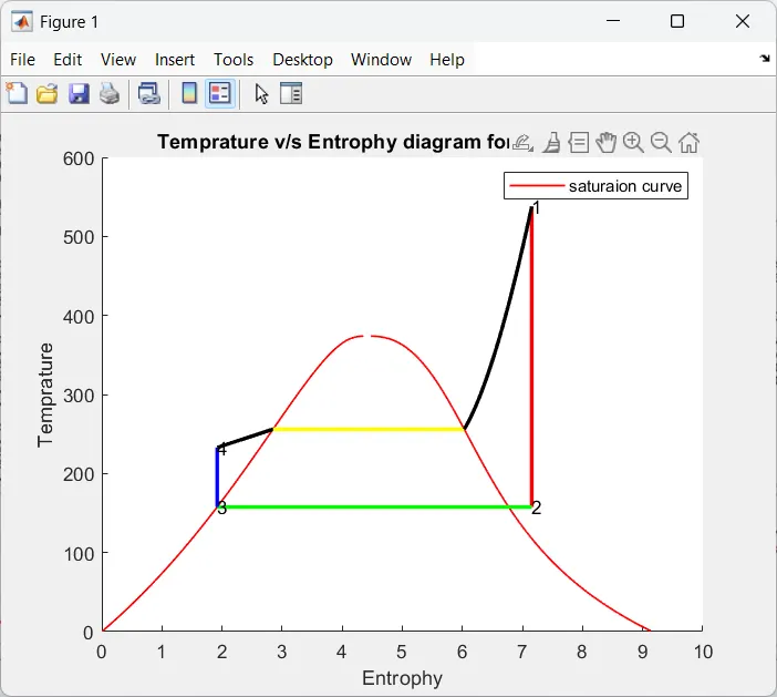
%plotting the T-S(Temprature v/s Entrophy) plot
figure(1)
hold on
plot(sf,T,'r','linewidth',1)
plot(sg,T,'r','linewidth',1)
plot([s1 s2],[T1 T2],'linewidth',2,'color','r')
plot([s2 s3],[T2 T3],'linewidth',2,'color','g')
plot([s3 s4],[T3 T4],'linewidth',2,'color','blue')
plot([s4 s5],[T4 T5],'linewidth',2,'color','black')
plot([s5 s6],[T5 T6],'linewidth',2,'color','y')
sc1=linspace(s6,s1,1000);
for l=1:length(sc1)
Tc1(l)=XSteam('T_ps',p1,sc1(l));
end
plot(sc1,Tc1,'k','linewidth',2)
%Markings
text(s1,T1,'1')
text(s2,T2,'2')
text(s3,T3,'3')
text(s4,T4,'4')
title('Temprature v/s Entrophy diagram for rankine cycle')
xlabel('Entrophy')
ylabel('Temprature')
legend('saturaion curve')
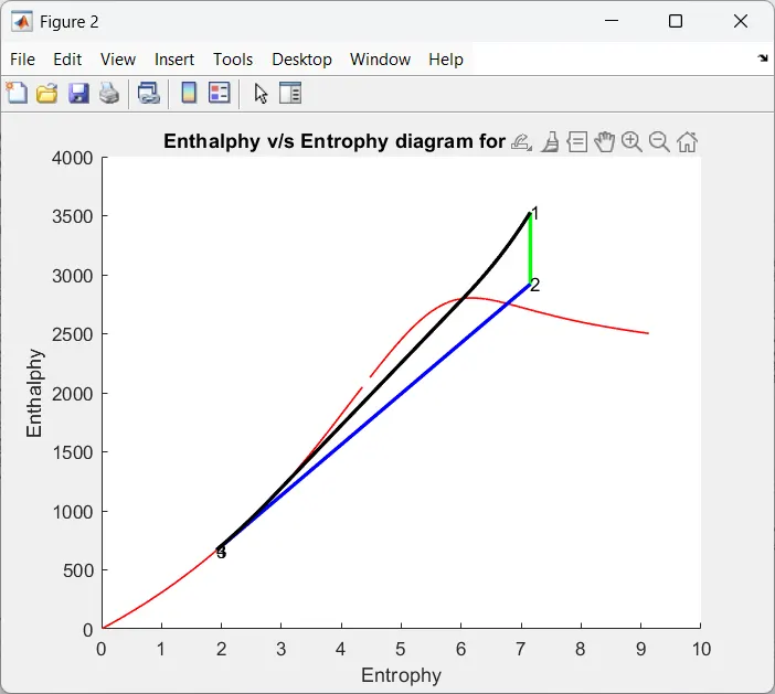
%plotting the H-S(Enthalphy v/s Entrophy) plot
figure(2)
hold on
plot(sf,hf,'r','linewidth',1)
plot(sg,hg,'r','linewidth',1)
plot([s1 s2],[h1 h2],'linewidth',2,'color','g')
plot([s2 s3],[h2 h3],'linewidth',2,'color','b')
plot([s3 s4],[h3 h4],'linewidth',2,'color','g')
hc=linspace(h4,h5,100);
for k=1:length(hc)
sch(k)=XSteam('s_ph',p1,hc(k));
end
plot(sch,hc,'k','linewidth',2)
plot([s5 s6],[h5 h6],'k','linewidth',2)
for m=1:length(sc1)
hc1(m)=XSteam('h_ps',p1,sc1(m));
end
plot(sc1,hc1,'k','linewidth',2)
%Markings
text(s1,h1,'1')
text(s2,h2,'2')
text(s3,h3,'3')
text(s4,h4,'4')
title('Enthalphy v/s Entrophy diagram for rankine cycle')
xlabel('Entrophy')
ylabel('Enthalphy')
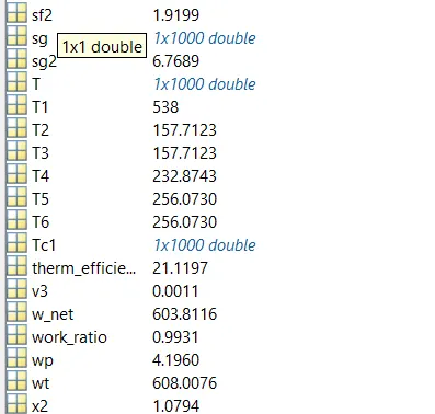
Explanation:

Conclusion:
- Rankine Cycle Simulator is created using MATLAB.
- The Net work output, Back work ratio is calculated.