Project 2 - Rankine cycle Simulator
AIM: To create a Rankine cycle simulator using matlab.
OBJECTIVE:
- To calculate the state points of the Rankine Cycle based on user inputs.
- Plotting the corresponding T-s and h-s plots for the given set of inputs.
- To explain the working of a rankine cycle simulator.
THEORY:
- The Rankine cycle is also called the Rankine vapor cycle which is a thermodynamic cycle that converts heat into mechanical energy. The Rankine cycle is named after William Johnson Macquorn Rankine, a 19th century Scottish engineer and physicist known for his research in the thermodynamic properties of steam.
- The Rankine cycle makes practical use of the increase in pressure that occurs when a condensed fluid is forced to evaporate within a contained vessel. The cycle begins when a fluid, such as water, is compressed and put under high pressure.
- When the liquid is heated, the compressed fluid becomes a vapor that can be used to generate mechanical energy. When the heat is reduced, the vapor cools and condenses back to liquid form. The cycle then begins again.
- A system that uses the Rankine cycle has four parts: a pump, a boiler, a turbine and a condenser. The pump's job is to deliver liquid to the boiler. The boiler's job is to heat the liquid and turn it to vapor. The vapor is then used to power a turbine. The turbine's job is to transform the energy created by the heated fluid into usable energy. The vaporized liquid is then cooled back to liquid state in the condenser. The pump pressurizes the liquid in the condenser and the cycle continues.
Basic Rankine Cycle Simulator
RANKINE CYCLE PROCESSES :
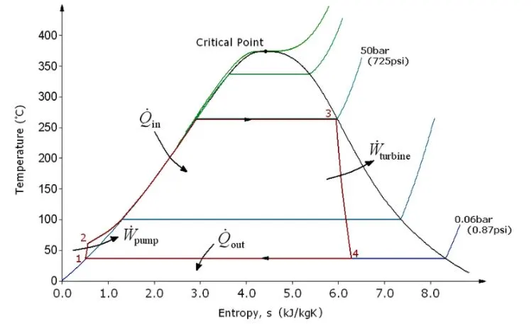
The four processes of an ideal Rankine cycle are as follows;
- Process 1-2: Isentropic compression in a pump. Here the working fluid is pumped from low to high pressure.
- 2-3: Constant pressure heat addition in the boiler. In this process, the high-pressure liquid is added to the boiler and is heated at constant pressure to become a dry saturated vapour.
- 3-4: Isentropic expansion in a turbine. The dry saturated vapour expands through the turbine resulting in the generation of power.
- 4-1: Constant pressure heat rejection in a condenser. Wet vapour is condensed at a constant pressure to become a saturated liquid.
MATLAB CODE:
% Program for Rankine Cycle Simulator

disp(' RANKINE CYCLE ');
disp('1-2 is isentropic expansion in turbine;');
disp('2-3 is constant pressure heat removal');
disp('3-4 is isentropic compression in pump');
disp('4-1 is constant pressure heat addition in boiler');

% Inputs
p1=input('Enter the pressure at turbine inlet(bar):');
T1=input('Enter the temperature at turbine inlet(degree C):');
p2=input('Enter the pressure at condenser inlet(bar):');

% Calculating dryness fraction at point 1
h1=XSteam('h_pT', p1, T1);
s1=XSteam('s_pT',p1 ,T1);

% At state 2
s2=s1; % Isentropic expansion
sf2=XSteam('sL_p' , p2);
sg2=XSteam('sV_p', p2);
sfg2=sg2-sf2;
x2=(s2-sf2)/(sg2-sf2);
hf2=XSteam('hL_p', p2);
hg2=XSteam('hV_p', p2);
hfg2=hg2-hf2;
h2=hf2+(x2*hfg2);

% At state point 3
p3=p2;
s3=XSteam('sL_p',p3);
h3=XSteam('hL_p',p3);

% At state point 4
s4=s3;
p4=p1;

% Work done by turbine
wt=h1-h2;

% Work done to run a pump
v3=XSteam('vL_p',p3);
wp=v3*(p4-p3)*100;
h4=h3+wp;

% Net work
Wnet=wt-wp;

%Heat into the system
Qin = h1 - h4;
%Heat out of the system
Qout = h2 - h3;

%Thermal efficiency
Thermal_eff =(Wnet/Qin)*100;

%Specific Steam Consumption
%SSC = mass flow rate/power
SSC =(3600/Wnet);
% Back work ratio
BW=(wp/wt)
%Calculating temperatures at the state points
T3 = XSteam ('Tsat_p', p3 );
T2 = T3;
Cp4 = XSteam ('Cp_ps', p4, s4);
Cv4 = XSteam ('Cv_ps', p4, s4);
k = Cp4/Cv4;
T4 = T3/((p3/p4)^((k-1)/k));


%Calculating temperature , entropy and enthalpy at the vapour and liquid
%line for plotting
T6 = XSteam ('Tsat_p',p1);
s5 = XSteam ('sL_p',p1);
s6 = XSteam ('sV_p',p1);
h5 = XSteam ('hL_p',p1);
h6 = XSteam ('hV_p',p1);
T5 = T6;

%Plotting the saturation curve
T =linspace(1,375,1000);
for i =1:length(T)

sf(i) = XSteam ('sL_T', T(i));
sg(i) = XSteam ('sV_T', T(i));
hf (i) = XSteam ('hL_T', T(i));
hg (i) = XSteam ('hV_T', T(i));
end

%Plotting T-s diagram
figure(1)
hold on
plot(sf,T,'r','LineWidth',1)
plot(sg, T, 'r','linewidth',1)
plot([s1 s2],[T1 T2],'b','LineWidth',2)
plot([s2 s3], [T2 T3] ,'b', 'linewidth', 2)
plot([s3 s4], [T3 T4], 'b', 'linewidth', 2)
plot([s4 s5],[T4 T5],'b','linewidth',2)
plot([s5 s6], [T5 T6], 'b', 'linewidth', 2)
sc1 = linspace (s6, s1, 1000);
for l = 1:length(sc1);
Tcl (l) = XSteam ('T_ps', p1, sc1(l));
end
plot(sc1, Tcl, 'k', 'linewidth', 2)
text(s1+0.1,T1,'1')
text(s2+0.1,T2,'2')
text (s3,T3-20,'3')
text (s4,T4+20,'4' )
title ('Temp vs Entropy plot');
xlabel ('Entropy (Kj/kgk) ')
ylabel ('Temperature (degree C) ');
legend ('Saturation curve');

%Plotting h-s diagram
 figure(2)
hold on
plot(sf,hf,'k','linewidth',1)
plot(sg, hg,'k','linewidth',1)
plot([s1 s2],[h1 h2],'r','lineWidth',2)
plot([s2 s3],[h2 h3],'r','lineWidth',2)
plot([s3 s4],[h3 h4],'r','lineWidth',2)
hc= linspace (h4, h5, 100);
for k =1:length(hc)
sch(k)=XSteam('s_ph',p1,hc(k));
end
plot(sch,hc,'r','lineWidth',2)
plot([s5 s6],[h5 h6],'r','LineWidth',2)


title ('Enthalpy vs Entropy plot')
xlabel ('Entropy , S (KJ/kgk) ')
ylabel ('Enthalpy , H (KJ/kg)')
legend('Saturation Curve','location','northwest')

%Results

disp('At stage point l');
nl = sprintf('P1 lS %.3f bar' ,p1);
disp(nl);
n2 = sprintf('Tl is %.3f C',T1);
disp(n2);
n3 = sprintf('hl is %.3f kJ/kg',h1);
disp (n3);
n4 = sprintf('sl is %.3f kJ/kgK',s1);
disp (n4);
disp ('At stage point 2');
nll = sprintf('P2 lS %.3f bar' ,p2);
disp(nll);
n21 = sprintf('T2 is %.3f C',T2);
disp (n21);
n31 = sprintf('h2 is %.3f kJ/kg',h2);
disp (n31);
n41 = sprintf('s2 is %.3f kJ/kgK',s2);
disp(n41);
disp('At stage point 3');
nl2 = sprintf('P3 is %.3f bar',p3 );
disp(nl2);
n22 = sprintf('T3 is %.3f C',T3);

n32 = sprintf('h3 is %.3f kJ/kg',h3);
disp (n32);
n42 = sprintf('s3 lS %.3f kJ/kgK',s3);
disp(n42);
disp ('At state point 4') ;
n13 = sprintf('P4 is %.3f bar',p4);
disp (n13);
n23 = sprintf('T4 lS %.3f C',T4);
disp (n23);
n33 = sprintf('h4 is %.3f kJ/kg',h4);
disp (n33);
n43 = sprintf('s4 lS %.3f kJ/kgK',s4);
disp(n43);
n14 = sprintf('Wt is %.3f kJ/kg',wt);
disp (n14);
n15 = sprintf('Wp is %.3f kJ/kg',wp);
disp (n15);
n16 = sprintf('Wnet is %.3f kJ/kg',Wnet);
disp (n16);
n17 = sprintf('Thermal_efficiency is %.2f percent',Thermal_eff)
disp (n17);
n18 = sprintf('SSC is %.2f kg/kWh',SSC);
disp (n18);
n19 = sprintf('Back WorkRatio is %.3f',BW)
COMMAND WINDOW OUTPUT:
>> Rankinecycle
 RANKINE CYCLE
1-2 is isentropic expansion in turbine;
2-3 is constant pressure heat removal
3-4 is isentropic compression in pump
4-1 is constant pressure heat addition in boiler
Enter the pressure at turbine inlet(bar):30
Enter the temperature at turbine inlet(degree C):400
Enter the pressure at condenser inlet(bar):0.05

BW =

    0.0027

At stage point l
P1 lS 30.000 bar
Tl is 400.000 C
hl is 3231.571 kJ/kg
sl is 6.923 kJ/kgK
At stage point 2
P2 lS 0.050 bar
T2 is 32.875 C
h2 is 2110.708 kJ/kg
s2 is 6.923 kJ/kgK
At stage point 3
P3 is 0.050 bar
h3 is 137.765 kJ/kg
s3 lS 0.476 kJ/kgK
At state point 4
P4 is 30.000 bar
T4 lS 36.935 C
h4 is 140.776 kJ/kg
s4 lS 0.476 kJ/kgK
Wt is 1120.863 kJ/kg
Wp is 3.011 kJ/kg
Wnet is 1117.852 kJ/kg

n17 =

    'Thermal_efficiency is 36.17 percent'

Thermal_efficiency is 36.17 percent
SSC is 3.22 kg/kWh

n19 =

    'Back WorkRatio is 0.003'
MATLAB PROCEDURE:
- Initially,we start with clear all ,close all and clc to clear all the previous data in the workspace.
- XSteam data is used to extract the steam and water properties of entropy and enthalpy and specific pressure and temperature for saturated liquid and saturated vapour conditions. .
- Now we have to start with inputting the input pressure at state point 1,Temperature at state point 1 and condenser inlet temperature at state point 2.
- Then all the state points are calculated with the help of XSteam data file and the inputs provided.
- Xsteam data works as ,h1=XSteam('h_pt',p1,T1) which return the enthalpy of water at given pressure and temperature in bar and degree C respectively.
- With the help of thermodynamic relation we find further state points and extract the data from Xsteam data file.
- f stands for saturated liquid and g stands for saturated vapour.
- Now we calculate the efficiency and Specific steam consumption of the rankine cycle from the thermodynamic relations.
- T, s and h are extracted at vapour and liquid line for plotting after 4th point for the variation in the plot.
- Saturation curve is plotted in red for saturated liquid and saturated gas in T-S and in H-S it is black.
- Plot for temperature vs entropy and enthalpy vs entropy is plotted with all the points obtained in the program.
- Results of the program is displayed in command window using sprintf command.
OUTPUT PLOTS:
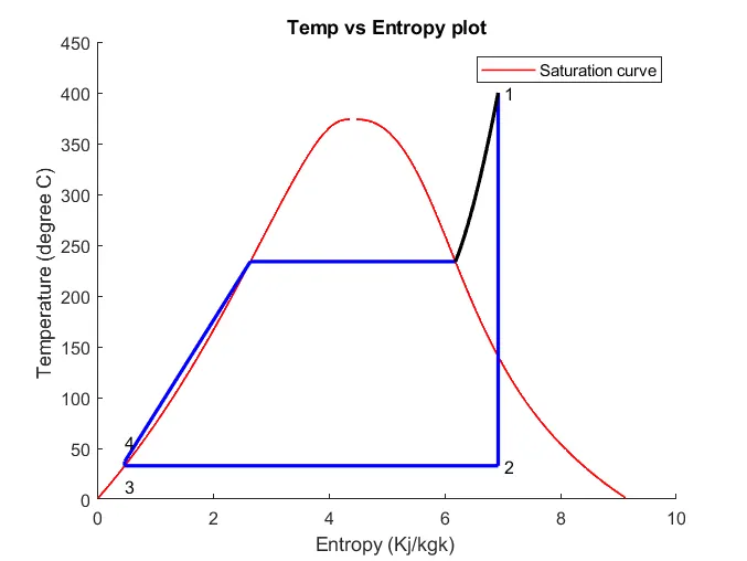
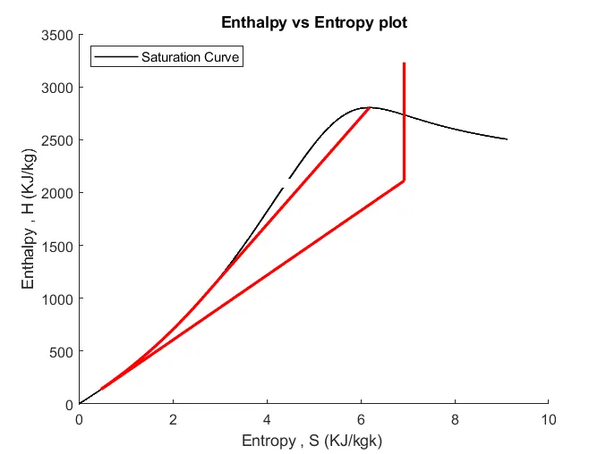
RESULTS:
- Thus with the help of matlab rankine cycle simulator is obtained where the values are extracted from 'XSteam' data file and the result is obtained from the given values of input.
- Net work done is 1117.852 KJ/KG.
- Thermal efficiency is 36.17%.
- Back work ratio is 0.003.
REFERENCES: