Air Standard Cycle
TITLE: Air standard cycle
AIM: To write a matlab program for solving otto cycle and create a plot for otto cycle.
OBJECTIVE:
(i) To write a matlab program to create a PV diagram for otto cycle.
(ii) To calculate the thermal efficiency of the engine.
THEORY:
- The air-standard-Otto cycle is an idealized cycle for the spark-ignition internal combustion engines.
- Otto cycle describes how an internal combustion engine which firstly converts the fuel’s chemical energy into thermal energy and then thermal energy into mechanical power, which is further used to move a vehicle.
- The air standard otto cycle has four processes to form a complete cycle, and the following assumptions are considered:-
(1). Air which is a working fluid throughout the cycle acts as an ideal gas.
(2). Combustion processes in otto cycle are replaced by heat addition processes at constant volume.
(3). Exhaust process is replaced by a heat rejection process at constant volume.
(4). As air is assumed to be an working fluid in the cycle ,constant values of specific heat at constant volume and pressure are assumed.
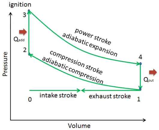
Figure.(1)- P-V Diagram of otto cycle
Otto cycle is made up of the following four internally reversible processes:
- Process 0-1 : Intake stroke
- Process 1-2 : Isentropic compression
- Process 2-3 : Constant-volume heat addition
- Process 3-4 : Isentropic expansion
- Process 4-1 : Constant-volume heat rejection
- The above PV diagram represents that the ideal Otto cycle represents how the volume and pressure of the air-fuel mixture changes due to the compression and expansion process.
- It clearly represents that when the piston performs work on the air-fuel mixture, the volume of the gas is compressed and substantially the pressure increases. Similarly, after the combustion process the heat released by the fuel/air mixture performs work on the piston due to which it expands.
- The above animation shows the working of otto cycle.
- Process 0-1 is an intake stroke in which the mass of working fluid is drawn into the cylinder at constant atmospheric pressure through the intake valve and the exhaust valve is kept closed during this process.
- Process 1-2 is an adiabatic compression stroke in which the piston moves from bottom dead centre to top dead centre.This is an isentropic compression process which states that there is no loss of mechanical energy due to friction.
- Process 2-3 is an ignition phase in which the piston is momentarily at rest position at top dead centre and this process represents the ignition of the fuel-air mixture and the subsequently burning rapidly.
- Process 3–4 is an adiabatic expansion (power stroke) in which the increased high pressure exerts a force on the piston and pushes it towards the bottom dead centre.
- Process 4–1 is an heat rejection phase in which the cycle is completed at constant volume and the heat is rejected while the piston is at bottom dead center.
- Process 1–0 is an exhaust stroke in which the gaseous mixture is emitted out to the atmosphere and the process starts again.
How to increase the efficiency of the Otto cycle?
- In order to increase the efficiency of otto cycle it has to be operated on lean fuel which is a fuel/air mixture containing relatively low proportion of fuel.
- It can also be improved by increasing the compression ratio which allows an engine to extract more mechanical energy from a given mass of air/fuel mixture.
PROCEDURE FOR MATLAB PROGRAM:
- Initially to start with the matlab program we need to assume temperature(t1) and pressure(p1) which is 500k and 101325 Pascal respectively.Gamma is a constant assumed as 1.4.
- Now engine geometric parameters which are bore,stroke,length of connecting rod and compression ratio are to be assumed.
- Next, we need to calculate the swept volume which is the volume swept by the engine piston during one stroke and the clearance volume which is the volume between the cylinder head and the piston when the piston is at top dead centre by using a formula. (i). Swept Volume=π/4*bore^2*stroke (ii). Clearance volume=swept volume/(compression ratio -1)
- We have v1 which is sum of swept volume and clearance volume and v2 which represents volume at top dead centre.
- To calculate the pressure at point 2 we have the equation for isentropic compression (i.e) p1v1^gamma=p2v2^gamma through which we can calculate the p2.
- After knowing the value for pressure at point 2 we can calculate the temperature at point 2 by using ideal gas law (P1V1/T1=P2V2/T2).
- Next the variables at state point 3 are calculated which represents the end of heat addition process at constant volume.As this process is at constant volume ,hence (V3=V2).Temperature at point 3 is assumed as 2300k.
- Now we can calculate pressure at point 3 by using ideal gas equation.
- Finally we need to find out the values for variables at state point 4, which represents the constant volume heat rejection process.Therefore (V4=V1).
- Now we can find pressure at state point 4 by using the formula (P4V4^Gamma=P3V3^Gamma) and similarly temperature at point 4 can be found by using (P3V3/T3=P4V4/T4).
- To calculate thermal efficiency of engine we can find it by using the formula Thermal efficiency=(1-1/(cr)^(gamma-1))*100 where ,cr represents the compression ratio.
- In order to plot the P-V diagram we have to use plot command and input the variables as required for plotting.
- For providing the name for x-axis and y-axis we use the command xlabel and ylabel respectively.
- As we cannot join the curve of compression and expansion stage in the P-V diagram.we have to understand the concept of piston kinematics.
- Now we have to write a new matlab program to determine the volume information during the compression and expansion stroke.
- To plot the compression and expansion stroke correctly we should know the thermodynamic relationship during compression and expansion stroke and the piston kinematics to find the volume change from tdc to bdc.
- Now we will use the formula to know the change in volume inside the combustion chamber. `V/V_c=1+1/2*(cr-1)[R+1-cos(theta)-(R^2-sin^2(theta))^0.5]`
- Now we will use function command which can be used whenever required and will save the script by the name engine kinematics(bore,stroke,con_rod,cr,start_crank,end_crank).
- Next we will call the function in command window and input the value of variables.
- We can input the value of v_compression - p_compression and and v_expansion -p_expansion.
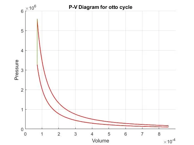
- Finally we can plot the exact PV diagram for otto cycle.
MATLAB PROGRAM:
% writing a matlab program for calculating the thermal efficiency and plotting pv diagram for otto cycle
clear all
close all
clc
% state variables at state point 1
p1=101325
t1=500
gamma=1.4;
% Engine geometric parameteres
bore=0.1;
stroke=0.1;
con_rod=0.15;
cr=12;
% Formula for swept volume and clearance volume
v_swept=(pi/4)*bore^2*stroke
v_clearance=v_swept/(cr-1)
v1=v_swept+v_clearance
v2=v_clearance

% state variables at state point 2
% p1v1^gamma=p2v2^gamma which is isentropic compression process
p2=p1*(v1/v2)^gamma

% Temperature at point 2 can be calculated by using ideal gas law
t2=p2*v2*t1/(p1*v1)

c_constant=p1*v1^gamma;
v_compression=engine_kinematics(bore,stroke,con_rod,cr,180,0);
p_compression=c_constant./v_compression.^gamma;

% state variables at state point 3
% at state point 3 it is constant volume combustion process .hence (v3=v2)
v3=v2;
t3=2300;

% pressure at state point 3 can be calculated using ideal gas law
p3=p2*(t3/t2);
c_constant=p3*v3^gamma
v_expansion=engine_kinematics(bore,stroke,con_rod,cr,0,180)
p_expansion=c_constant./v_expansion.^gamma

% state variable at state point 4
% constant volume heat rejection.hence(v4=v1)
v4=v1;

%p3v3^gamma=p4v4^gamma
p4=p3*(v3/v4)^gamma
t4=p4*v4*t3/(p3*v3)

% efficiency for otto cycle
thermal_efficiency=(1-1/(cr)^(gamma-1))*100
figure(1)
hold on
plot(v_compression,p_compression,'LineWidth',1,'Color','r')
plot(v_expansion,p_expansion,'LineWidth',1,'Color','r')
plot(v1,p1,'linewidth',1,'Color','r')
plot(v2,p2,'linewidth',1,'Color','r')
plot([v2 v3],[p2 p3],'linewidth',1)
plot([v4 v1],[p4 p1],'linewidth',1)
plot(v3,p3,'linewidth',1,'Color','r')
plot(v4,p4,'linewidth',1,'Color','r')
title('P-V Diagram for otto cycle')
xlabel('Volume')
ylabel('Pressure')
grid on
OUTPUT:
p1 =

      101325


t1 =

   500


v_swept =

   7.8540e-04


v_clearance =

   7.1400e-05


v1 =

   8.5680e-04


v2 =

   7.1400e-05


p2 =

   3.2853e+06


t2 =

   1.3510e+03


R =

    3.0000


theta =

  Columns 1 through 15

  180.0000  178.4874  176.9748  175.4622  173.9496  172.4370  170.9244  169.4118  167.8992  166.3866  164.8739  163.3613  161.8487  160.3361  158.8235

  Columns 16 through 30

  157.3109  155.7983  154.2857  152.7731  151.2605  149.7479  148.2353  146.7227  145.2101  143.6975  142.1849  140.6723  139.1597  137.6471  136.1345

  Columns 31 through 45

  134.6218  133.1092  131.5966  130.0840  128.5714  127.0588  125.5462  124.0336  122.5210  121.0084  119.4958  117.9832  116.4706  114.9580  113.4454

  Columns 46 through 60

  111.9328  110.4202  108.9076  107.3950  105.8824  104.3697  102.8571  101.3445   99.8319   98.3193   96.8067   95.2941   93.7815   92.2689   90.7563

  Columns 61 through 75

   89.2437   87.7311   86.2185   84.7059   83.1933   81.6807   80.1681   78.6555   77.1429   75.6303   74.1176   72.6050   71.0924   69.5798   68.0672

  Columns 76 through 90

   66.5546   65.0420   63.5294   62.0168   60.5042   58.9916   57.4790   55.9664   54.4538   52.9412   51.4286   49.9160   48.4034   46.8908   45.3782

  Columns 91 through 105

   43.8655   42.3529   40.8403   39.3277   37.8151   36.3025   34.7899   33.2773   31.7647   30.2521   28.7395   27.2269   25.7143   24.2017   22.6891

  Columns 106 through 120

   21.1765   19.6639   18.1513   16.6387   15.1261   13.6134   12.1008   10.5882    9.0756    7.5630    6.0504    4.5378    3.0252    1.5126         0


c_constant =

    8.7666


R =

    3.0000


theta =

  Columns 1 through 15

         0    1.5126    3.0252    4.5378    6.0504    7.5630    9.0756   10.5882   12.1008   13.6134   15.1261   16.6387   18.1513   19.6639   21.1765

  Columns 16 through 30

   22.6891   24.2017   25.7143   27.2269   28.7395   30.2521   31.7647   33.2773   34.7899   36.3025   37.8151   39.3277   40.8403   42.3529   43.8655

  Columns 31 through 45

   45.3782   46.8908   48.4034   49.9160   51.4286   52.9412   54.4538   55.9664   57.4790   58.9916   60.5042   62.0168   63.5294   65.0420   66.5546

  Columns 46 through 60

   68.0672   69.5798   71.0924   72.6050   74.1176   75.6303   77.1429   78.6555   80.1681   81.6807   83.1933   84.7059   86.2185   87.7311   89.2437

  Columns 61 through 75

   90.7563   92.2689   93.7815   95.2941   96.8067   98.3193   99.8319  101.3445  102.8571  104.3697  105.8824  107.3950  108.9076  110.4202  111.9328

  Columns 76 through 90

  113.4454  114.9580  116.4706  117.9832  119.4958  121.0084  122.5210  124.0336  125.5462  127.0588  128.5714  130.0840  131.5966  133.1092  134.6218

  Columns 91 through 105

  136.1345  137.6471  139.1597  140.6723  142.1849  143.6975  145.2101  146.7227  148.2353  149.7479  151.2605  152.7731  154.2857  155.7983  157.3109

  Columns 106 through 120

  158.8235  160.3361  161.8487  163.3613  164.8739  166.3866  167.8992  169.4118  170.9244  172.4370  173.9496  175.4622  176.9748  178.4874  180.0000


v_expansion =

   1.0e-03 *

  Columns 1 through 15

    0.0714    0.0716    0.0721    0.0730    0.0743    0.0760    0.0779    0.0803    0.0830    0.0861    0.0895    0.0932    0.0973    0.1017    0.1065

  Columns 16 through 30

    0.1116    0.1170    0.1227    0.1287    0.1350    0.1416    0.1485    0.1557    0.1631    0.1708    0.1787    0.1869    0.1953    0.2040    0.2128

  Columns 31 through 45

    0.2219    0.2311    0.2406    0.2502    0.2600    0.2699    0.2800    0.2902    0.3005    0.3109    0.3214    0.3320    0.3427    0.3535    0.3643

  Columns 46 through 60

    0.3752    0.3860    0.3970    0.4079    0.4188    0.4297    0.4407    0.4515    0.4624    0.4732    0.4840    0.4947    0.5053    0.5158    0.5263

  Columns 61 through 75

    0.5366    0.5469    0.5571    0.5671    0.5770    0.5868    0.5965    0.6060    0.6154    0.6247    0.6338    0.6427    0.6515    0.6601    0.6685

  Columns 76 through 90

    0.6768    0.6849    0.6928    0.7006    0.7081    0.7155    0.7227    0.7297    0.7366    0.7432    0.7497    0.7559    0.7620    0.7679    0.7736

  Columns 91 through 105

    0.7791    0.7844    0.7895    0.7945    0.7992    0.8037    0.8081    0.8123    0.8163    0.8201    0.8237    0.8271    0.8303    0.8333    0.8362

  Columns 106 through 120

    0.8389    0.8413    0.8436    0.8457    0.8477    0.8494    0.8510    0.8523    0.8535    0.8545    0.8553    0.8560    0.8564    0.8567    0.8568


p_expansion =

   1.0e+06 *

  Columns 1 through 15

    5.5931    5.5732    5.5141    5.4180    5.2884    5.1297    4.9468    4.7451    4.5298    4.3061    4.0783    3.8505    3.6258    3.4070    3.1959

  Columns 16 through 30

    2.9941    2.8025    2.6216    2.4517    2.2927    2.1444    2.0064    1.8783    1.7596    1.6496    1.5479    1.4538    1.3669    1.2865    1.2122

  Columns 31 through 45

    1.1435    1.0799    1.0211    0.9666    0.9161    0.8693    0.8259    0.7855    0.7480    0.7131    0.6806    0.6504    0.6222    0.5958    0.5712

  Columns 46 through 60

    0.5482    0.5267    0.5065    0.4876    0.4699    0.4532    0.4376    0.4229    0.4091    0.3961    0.3838    0.3722    0.3613    0.3510    0.3413

  Columns 61 through 75

    0.3321    0.3234    0.3152    0.3074    0.3000    0.2930    0.2864    0.2801    0.2741    0.2685    0.2631    0.2580    0.2532    0.2485    0.2442

  Columns 76 through 90

    0.2400    0.2360    0.2323    0.2287    0.2253    0.2220    0.2189    0.2160    0.2132    0.2105    0.2080    0.2056    0.2033    0.2011    0.1990

  Columns 91 through 105

    0.1971    0.1952    0.1934    0.1918    0.1902    0.1887    0.1872    0.1859    0.1846    0.1834    0.1823    0.1812    0.1803    0.1793    0.1785

  Columns 106 through 120

    0.1777    0.1770    0.1763    0.1757    0.1751    0.1746    0.1742    0.1738    0.1734    0.1732    0.1729    0.1727    0.1726    0.1725    0.1725


p4 =

   1.7251e+05


t4 =

  851.2465


thermal_efficiency =

   62.9893
PROGRAM FOR PISTON KINEMATICS:
function [v]=engine_kinematics(bore,stroke,con_rod,cr,start_crank,end_crank)
% a is crank pin radius
a=stroke/2;

% R is the ratio of connecting rod to crank pin radius
R=con_rod/a;
cr=12;

% Formula for swept volume and clearance volume
v_swept=(pi/4)*bore^2*stroke;
v_clearance=v_swept/(cr-1);
theta= linspace(start_crank,end_crank,120);

% formula for change in volume inside the engine combustion chamber
% V/Vc=1+(1/2)*(cr-1)[R+1-cos(theta)-(R^2-sin^2(theta)^0.5]
term1=0.5*(cr-1);
term2=R+1-cosd(theta);
term3=(R^2-sind(theta).^2).^0.5;
v=(1+term1*(term2-term3)).*v_clearance;
end
OUTPUT:
v_compression=engine_kinematics(0.1,0.1,0.15,12,0,180)

v_compression =

   1.0e-03 *

  Columns 1 through 15

    0.0714    0.0716    0.0721    0.0730    0.0743    0.0760    0.0779    0.0803    0.0830    0.0861    0.0895    0.0932    0.0973    0.1017    0.1065

  Columns 16 through 30

    0.1116    0.1170    0.1227    0.1287    0.1350    0.1416    0.1485    0.1557    0.1631    0.1708    0.1787    0.1869    0.1953    0.2040    0.2128

  Columns 31 through 45

    0.2219    0.2311    0.2406    0.2502    0.2600    0.2699    0.2800    0.2902    0.3005    0.3109    0.3214    0.3320    0.3427    0.3535    0.3643

  Columns 46 through 60

    0.3752    0.3860    0.3970    0.4079    0.4188    0.4297    0.4407    0.4515    0.4624    0.4732    0.4840    0.4947    0.5053    0.5158    0.5263

  Columns 61 through 75

    0.5366    0.5469    0.5571    0.5671    0.5770    0.5868    0.5965    0.6060    0.6154    0.6247    0.6338    0.6427    0.6515    0.6601    0.6685

  Columns 76 through 90

    0.6768    0.6849    0.6928    0.7006    0.7081    0.7155    0.7227    0.7297    0.7366    0.7432    0.7497    0.7559    0.7620    0.7679    0.7736

  Columns 91 through 105

    0.7791    0.7844    0.7895    0.7945    0.7992    0.8037    0.8081    0.8123    0.8163    0.8201    0.8237    0.8271    0.8303    0.8333    0.8362

  Columns 106 through 120

    0.8389    0.8413    0.8436    0.8457    0.8477    0.8494    0.8510    0.8523    0.8535    0.8545    0.8553    0.8560    0.8564    0.8567    0.8568
OUTPUT PLOTS:
PLOT(1)
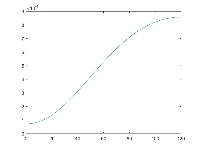
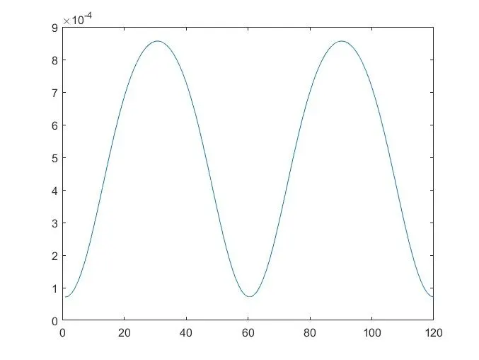
Crank angle vs volume Crank angle vs volume
PLOT(2) PLOT(3)
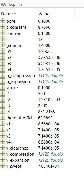
Workspace Output
Errors during programming:
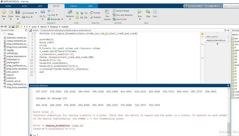
Error occurred because of not using element-wise operator.It was rectified by using element-wise operator.
CONCLUSION/RESULTS:
- Using the Matlab program,PV diagram for otto cycle has been plotted for the input variable.
- The thermal efficiency of otto cycle is 62.98%.
- The thermal efficiency can be improved by operating the engine on lean fuel and by increasing the compression ratio.
REFERENCES:
- Figure(1) is obtained from https://www.nuclear-power.com/nuclear-engineering/thermodynamics/thermodynamic-cycles/otto-cycle-otto-engine/otto-cycle-pv-ts- diagram/
- Animation of otto cycle is obtained from https://www.youtube.com/watch?v=CaVXe3Gxomo