Curve Fitting Using Matlab
TITLE: Curve fitting for Linear and Cubic polynomial.
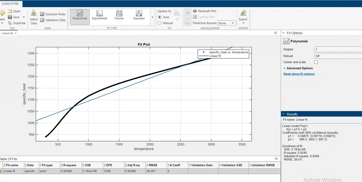
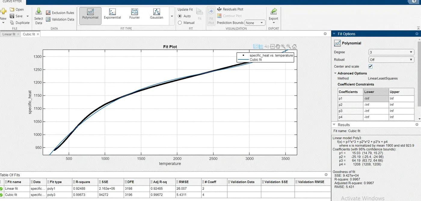
AIM: To Write a Matlab program to fit a linear and cubic polynomial for the Cp data and to plot the linear and cubic curve fit with the raw data points.
OBJECTIVES:
- To write a code and fit a linear and cubic polynomial for the Cp data.
- Plot the linear and cubic fit curves and compare it along with predicted specific heat.
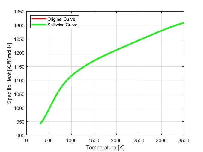
- Write a code to show splitwise method for the curve fitting.
- Various parameters used to measure the fitness characteristics of linear and cubic polynomial curve.
THEORY:
- Curve fitting is the process of finding a mathematical function in an analytic form that best fits this set of data.
- It can also be called as representation of a data spread by assigning a best fit function (curve) along the entire range. Ideally, it will capture the trend in the data and allow us to make predictions of how the data series will behave in the future.
- Curve fitting can involve either interpolation where a function is discovered that is an exact fit to the data points or smoothing where when we find a function that is an approximate fit to the data points and we give room for error and allow our actual points to be near, but not necessarily on the line; given the error is minimized overall.
- Matlab has two functions, polyfit and polyval, which can quickly and easily fit a set of data points with a polynomial.
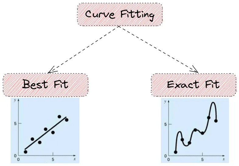
- Generally, curve fitting falls into two main categories based on how we handle the observed data:
(1).Best Fit
-
Here, we assume that the measured data points are noisy. So, we don’t want to fit a curve that intercepts every data point. Our goal is to learn a function that minimizes some predefined error on the given data points.
The simplest best fit method is linear regression, where the curve is a straight line. More formally, we have the parametric function `y=ax+b`weref `a` is the slope and `b` is the intercept and a set of samples`(x_1,y_1),(x_2,y_2)......(x_n,y_n)`Our goal is to learn the values of
 and
and  to minimize an error criterion on the given samples.
 -
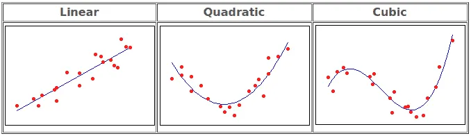
More generally, polynomial regression refers to the case that we want to fit a polynomial of a specific order `d` to our data:
- For Linear : `y=ax+b`
- For Quadratic : `y=ax^2+bx+c`
- For Cubic : `y=ax^3+bx^2+cx+d`
(2).Perfect Fit
-
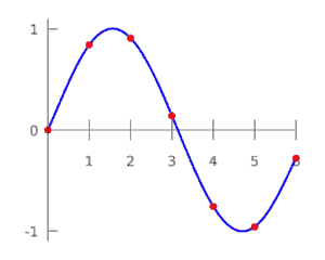
In this case, we assume that the given samples are not noisy, and we want to learn a curve that passes through each point. It is useful in cases we want to derive finite-difference approximations or to find minimums, maximums, and zero crossings of a function.
In the figure above, we can see an example of a perfect fit using polynomial interpolation.
Parameters used to measure the fitness characteristics for both the curves:
- The parameters used to measure the fitness of the curve is by knowing the goodness of fit statistically evaluated after using graphical methods. Curve Fitting Toolbox software supports these goodness-of-fit statistics for parametric models:
- The sum of squares due to error (SSE)
-
R-square
-
Adjusted R-square
-
Root mean squared error (RMSE)
- Sum of square due to error: It is also called the summed square of residuals i.e. the sum of square difference between the predicted value and the original data and is usually labeled as SSE. `SSE=sum_(i=1)^n[(y_i-f(x_i))^2]` A value closer to 0 indicates that the model has a smaller random error component, and that the fit will be more useful for prediction.
- R-Square: R-square is defined as the ratio of the sum of squares of the regression (SSR) and the total sum of squares (SST).`R^2=( SSR)/(SST)`
SST is called the sum of squares about the mean.
3. Adjusted R-Square: The adjusted R-square statistic is generally the best indicator of the fit quality when you compare two models that are nested i.e. a series of models each of which adds additional coefficients to the previous model.
`Adjusted R-Square=1-((SSE)(n-1))/(SST(v)`
The adjusted R-square statistic can take on any value less than or equal to 1, with a value closer to 1 indicating a better fit.
4.Root Mean Squared Error: This statistic is also known as the fit standard error and the standard error of the regression. It is an estimate of the standard deviation of the random component in the data.
`RMSE=sqrt((SSE)/n`
- How to make curve fit perfectly?
- Perfect fit means tracing the data points exactly through the original dataset which will make a perfect curve without any errors.
- SplitWise method makes the curve fit a perfect fit as every point in curve fit coincides with the original data, so by using splitwise method we can obtain a perfect curve fit.
- Perfect fit can also be obtained by increasing the degree of polynomial and tracing the curve through original curve.
- It can also be obtained by using polynomial interpolation in which the values are estimated between known datapoints.
- How to get the best fit?
- A more accurate way of finding the line of best fit is by using least square method .
- The least squares method is a statistical procedure to find the best fit for a set of data points by minimizing the sum of the offsets or residuals of points from the plotted curve.
- Least squares method provides the overall rationale for the placement of the line of best fit among the data points being studied.
- What could be done to improve the cubic fit?
- Cubic fit can be improved by using Splitwise method.
- In Splitwise method we split the data of specific heat in equal number of parts by which we can obtain a smooth curve and get the best cubic fit.
MATLAB PROGRAM FOR LINEAR CURVE:
% Write a matlab program for linear and cubic curve fitting
clear all
close all
clc
% Loading the data
cp_data= load('data');
temperature= cp_data(:,1);          % Temperature in kelvin
specific_heat= cp_data(:,2);        % Specific heat in KJ/Kmol-K

% For linear curve fit eqn is f(x)=ax+b
% Polyfit command is used to calculate the coefficients a,b
% Polyval command is used to calculate the predicted specific heat
co_efficient1=polyfit(temperature,specific_heat,1)
predicted_cp1=polyval(co_efficient1,temperature);

% Plot for linear curve fitting and comparing it with predicted cp
figure (1)
plot(temperature,specific_heat,'linewidth',3,'color','r')
hold on
plot(temperature,predicted_cp1,'linewidth',3,'color','b')
xlabel('Temperature [K]')
ylabel('Specific Heat [KJ/Kmol-K]')
legend('Original data set','Predicted data set',Location='northwest')
title('Linear Polynomial Curve Fitting')
grid on

% Calculating the goodness of fit for linear curve
m=mean(specific_heat)
error=specific_heat-predicted_cp1;
sse_linear=error.^2;
SSE_linear=sum(sse_linear);

ssr_linear=(predicted_cp1-m).^2;
SSR_linear=sum(ssr_linear);

SST_linear=SSR_linear+SSE_linear;

% Calculation of R_square
r_square_linear= (SSR_linear/SST_linear);

% Calculation of rmse
RMSE_linear=sqrt(SSE_linear/length(temperature));

if (r_square_linear>0.95)
    disp('Linear Curve fit is good')
else
    disp('Linear Curve fit is not Good')
end
OUTPUT WINDOW:
co_efficient1 =

    0.0988  995.2017


m =

   1.1828e+03

% Value of 0.95 and above for R-Square is considered a good fit
r_square_linear =

    0.9249

Linear Curve fit is not Good
>>
MATLAB PROGRAM FOR CUBIC CURVE:
% To write a Matlab program for cubic curve fitting
clear all
close all
clc

% Loading the data
cp_data=load('data');
temperature=cp_data(:,1);    % First column representign the data for temperature
specific_heat=cp_data(:,2);  % Second column representing the data for specific heat

% For cubic curve fit eqn is f(x)= a(x^3)+b(x^2)+c(x)+d
% Polyfit command is used to calculate the coefficients a,b,c,d
% Polyval command is used to calculate the predicted specific heat
co_efficient2=polyfit(temperature,specific_heat,3)
predicted_cp2=polyval(co_efficient2,temperature);

% Plot for cubic curve fitting and comparing it with predicted cp
figure (2)
plot(temperature,specific_heat,'LineWidth',3,'Color','r')
hold on
plot(temperature,predicted_cp2,'linewidth',3,'Color','b')
xlabel('Temperature [K]')
ylabel('Specific Heat [KJ/Kmol-K]')
legend('Original data set','Predicted data set',Location='northwest')
title('Cubic Polynomial Curve Fitting')
grid on


% for cubic curve
m=mean(specific_heat);
error=specific_heat-predicted_cp2;
sse_cubic=error.^2;
SSE_cubic=sum(sse_cubic);

ssr_cubic=(predicted_cp2-m).^2;
SSR_cubic=sum(ssr_cubic);

SST_cubic=SSR_cubic+SSE_cubic;

% Calculation of R_square
r_square_cubic= (SSR_cubic/SST_cubic);

% Calculation of rmse
RMSE_cubic=sqrt(SSE_cubic/length(temperature));

if (r_square_cubic>0.95)
    disp('Linear Curve fit is good')
else
    disp('Linear Curve fit is not Good')
end
OUTPUT WINDOW:
co_efficient2 =

    0.0000   -0.0001    0.3879  838.8966


r_square_cubic =

    0.9967

Linear Curve fit is good
>>
MATLAB PROGRAM FOR SPLITWISE METHOD:
% Writing a program for splitwise method for curve fitting
clear all
close all
clc

% Loading the data
cp_data=load('data');
temperature=cp_data(:,1);    % First column represents the temperature
cp=cp_data(:,2);             % Second column represents the specific heat

% Splitting the data for cubic curve
temperature1=cp_data(1:400,1);
cp1=cp_data(1:400,2);

temperature2=cp_data(401:800,1);
cp2=cp_data(401:800,2);

temperature3=cp_data(801:1200,1);
cp3=cp_data(801:1200,2);

temperature4=cp_data(1201:1600,1);
cp4=cp_data(1201:1600,2);

temperature5=cp_data(1601:2000,1);
cp5=cp_data(1601:2000,2);

temperature6=cp_data(2001:2400,1);
cp6=cp_data(2001:2400,2);

temperature7=cp_data(2401:2800,1);
cp7=cp_data(2401:2800,2);

temperature8=cp_data(2801:3200,1);
cp8=cp_data(2801:3200,2);

% Calculating the coefficients and specific heat for the splitted curve

[coefficient1,s,mu]=polyfit(temperature1,cp1,3);
predicted_cp1=polyval(coefficient1,temperature1,s,mu);

[coefficient2,s,mu]=polyfit(temperature2,cp2,3);
predicted_cp2=polyval(coefficient2,temperature2,s,mu);

[coefficient3,s,mu]=polyfit(temperature3,cp3,3);
predicted_cp3=polyval(coefficient3,temperature3,s,mu);

[coefficient4,s,mu]=polyfit(temperature4,cp4,3);
predicted_cp4=polyval(coefficient4,temperature4,s,mu);

[coefficient5,s,mu]=polyfit(temperature5,cp5,3);
predicted_cp5=polyval(coefficient5,temperature5,s,mu);

[coefficient6,s,mu]=polyfit(temperature6,cp6,3);
predicted_cp6=polyval(coefficient6,temperature6,s,mu);

[coefficient7,s,mu]=polyfit(temperature7,cp7,3);
predicted_cp7=polyval(coefficient7,temperature7,s,mu);

[coefficient8,s,mu]=polyfit(temperature8,cp8,3);
predicted_cp8=polyval(coefficient8,temperature8,s,mu);


% Comapre the curve fit with original data
plot(temperature,cp,'linewidth',3,'color','r')
hold on
plot(temperature1,predicted_cp1,'linewidth',3,'color','g')
plot(temperature2,predicted_cp2,'linewidth',3,'color','g')
plot(temperature3,predicted_cp3,'linewidth',3,'color','g')
plot(temperature4,predicted_cp4,'linewidth',3,'color','g')
plot(temperature5,predicted_cp5,'linewidth',3,'color','g')
plot(temperature6,predicted_cp6,'linewidth',3,'color','g')
plot(temperature7,predicted_cp7,'linewidth',3,'color','g')
plot(temperature8,predicted_cp8,'linewidth',3,'color','g')
xlabel('Temperature [K]')
ylabel('Specific Heat [KJ/Kmol-K]')
legend('Original Curve','Splitwise Curve',Location='northwest')
grid on
STEPWISE CODE EXPLANATION:
- Firstly starting the program with three basic command i.e clear all, close all, clc which clears all the data stored in the previous program ,clears all the plots and clears the command window.
- Now we have a dataset which has to be loaded in the program by using load command and calling it by name inside the parenthesis.
- Dataset has values of temperature and specific heat and the first column represents the temperature ,Similarly the second column represents the specific heat.
- Data loaded is assigned to a variable 'cp_data' which is stored in workspace and it can be called whenever required in the main program.
- Now in order to perform curve fitting it can be done using two commands that are polyfit and polyval.
- Polyfit command is used to determine the value of coefficients for both linear and cubic curve.It is a Matlab function that computes a least squares polynomial for a given set of data.
- Polyval command is used to evaluate a polynomial for a given set of x values. So, Polyval generates a curve to fit the data based on the coefficients found using polyfit.
- Next by using plot command a plot of temperature and specific heat is plotted and then it is compared with the predicted dataset.
- After running the program we can see that the plot obtained has variation between curve fit and the original dataset, So in order to obtain the perfect fit we have to increase the degree of polynomial.
- xlabel and ylabel command is used to label the axis and the legend command is used to differentiate curve obtained on the graph.
- Now the goodness of the fit can be evaluated by checking the sum of square due to error(SSE),R-Square,Adjusted R-Square and root mean squared error (RSME).
- R-square is the best method for evaluating the goodness of fit for this program and the value of R-Square above 0.95 is considered for a good fit.
- Similar program is used for cubic curve in which the degree of polynomial is increased to 3 to obtain a smooth curve.
- As we increase the degree of polynomial the equation is badly conditioned and it can be corrected by scaling and centering the equation and we can see that value for R-Square obtained for cubic curve is 0.99 which is considered a value for good fit.
- Finally Splitwise method is used for curve fitting in which the dataset is splited in 8 equal parts and it can seen that using splitwise method the most perfect fit is obtained.The curve passes through each and every data point of the original dataset and hence it is the most effective way of curve fitting.
ERRORS DURING THE PROGRAM:
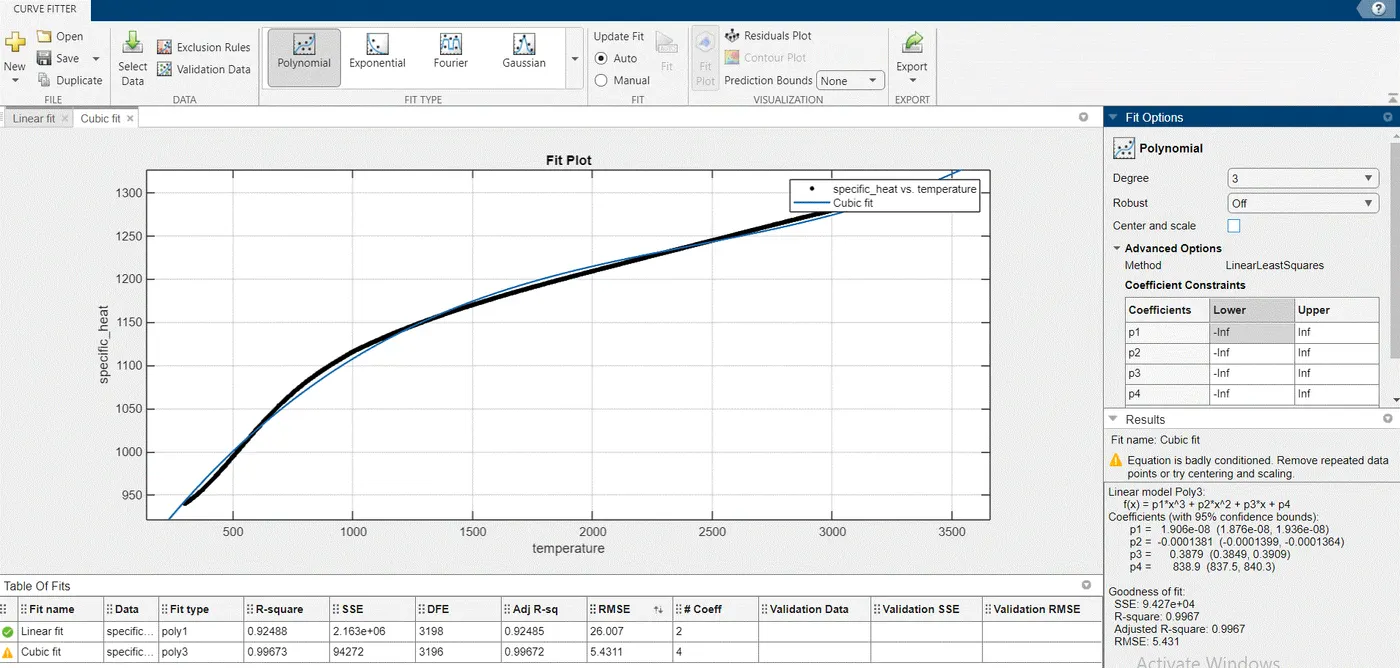
- The curve fit box displays in the results section that the equation is badly conditioned which is due to increasing the degree of polynomial and this can be rectified by centering and scaling.
OUTPUT/RESULTS:
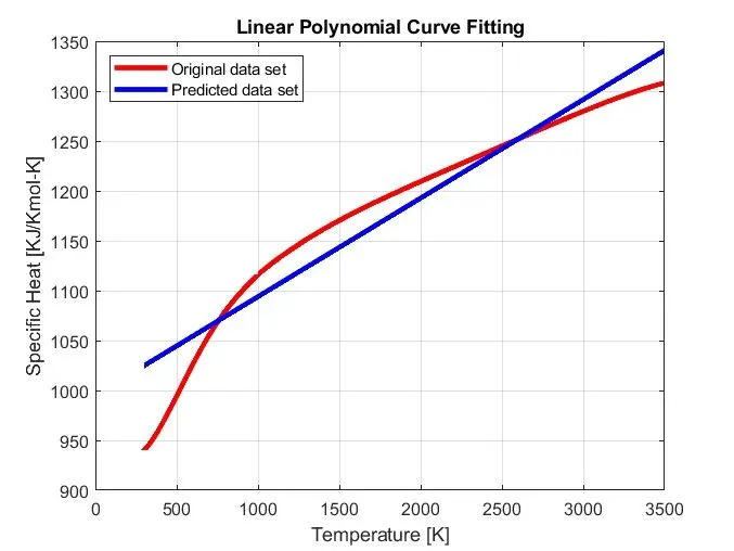
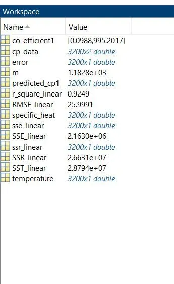
Fig(Linear Curve fit) Workspace for Linear curve 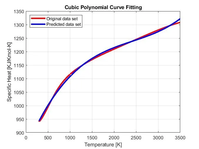
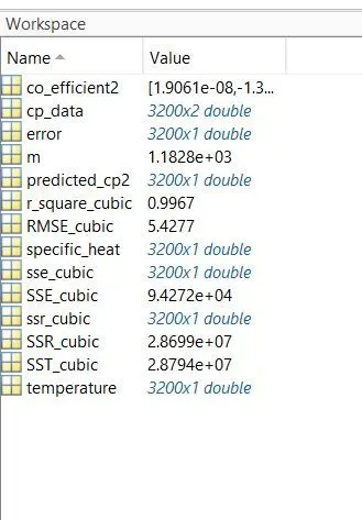
Fig(Cubic Curve Fit) Workspace for Cubic curve
Fig(Splitwise Curve)
(Linear Curve Fit in Curve Fitter Toolbox)
(Cubic Curve Fit in Curve Fitter Toolbox)
CONCLUSION:
- It can be concluded that there are various ways for fitting the curve through which a perfect fit of curve can be obtained.
- Curve can be fitted with perfect fit by increasing the degree of polynomial which also results in bad conditioning of equation and it can be rectified by centering and scaling.
- Splitwise method for curve fitting results in the perfect fit of the curve with the original curve tracing the curve exactly through each and every point of the original dataset.
REFERENCES: