Week 3 - Solving second order ODEs

TITLE: Solving Second Order Differential Equation.

AIM : To Write a Matlab Program to Solve an Second Order Ordinary Differential Equation and Animate the Motion Of Simple Pendulum.

OBJECTIVE:

• To solve the following ODE which represents the equation of motion of a simple pendulum with damping

`(d^2theta)/dt^2+b/m*(d theta)/dt+g/l*sin theta=0`

• To Create an animation of motion of simple pendulum.
• To Create a plot for angular displacemtent and velocity w.r.t. time.

THEORY:

• A pendulum is a weight suspended from a fixed pivot so that it can swing freely making a motion .When a pendulum is displaced sideways from its equilibrium position, it is subjected to a restoring force which is due to the gravity, that will accelerate it back toward the equilibrium position. When released, the restoring force acting on the pendulum's mass causes it to oscillate about the equilibrium position, swinging back and forth from the fixed pivot.
• When the pendulum swings back and forth along a single line that means it is performing simple harmonic motion.
• The motion of the pendulum is dependent on the Newtons second law of motion. Through this law, we get a second order Ordinary Differential Equation that describes the position of the 'ball' w.r.t time.
• Newton's second law of motion describes a simple relationship between the acceleration of an object with mass m, and the net force acting on that object.
• One end of pendulum is fixed and the other end moves according to the solution obtained from the Ordinary differential equation.

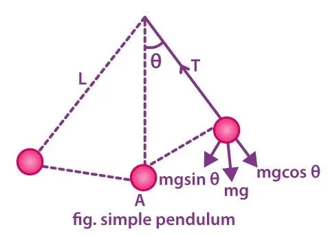
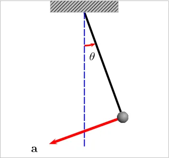
Animation of Simple Pendulum

GOVERNING EQUATION:

• ODE representing the equation of motion of a simple pendulum with damping is `(d^2theta)/dt^2+b/m*(d theta)/dt+g/l*sin theta=0` -----------(1) Where,

  g = gravity in m/s2,

  L = length of the pendulum in m,

  m = mass of the ball in kg,

  b=damping coefficient.

• In order to solve the ODE ,We have to break second order ode into two first order ODE,
• We can assume `theta=theta_1`
• So `(d theta)/dt=(d theta_1)/dt=theta_2` --------(2)
• Similarly,`(d^2 theta)/dt^2=(d^2 theta_1)/dt^2=d/dt*((d theta_1)/dt)=d/dt*theta_2` ----(3)
• `(d^2theta_1)/dt^2+b/m*(d theta_1)/dt+g/l*sin theta_1=0` ---- Inputing the value of theta (4)
• `(d theta_2)/dt+b/m*theta_2+g/l*sin theta_1=0` ----(5)
• `(d theta)/dt=(d theta_1)/dt=theta_2` ----(First order ODE)
• `(d theta_2)/dt=-b/m*theta_2-g/l*sin theta_1` ----(Second order ODE)

MATLAB PROGRAM FOR DEFINING A FUNCTION:

function [dtheta_dt]= ode_function(t,theta,b,g,l,m)

theta1=theta(1);
theta2=theta(2);

% Breaking second order ODE into two single order ODE
dtheta1_dt=theta2;
dtheta2_dt=-(b/m)*theta2-(g/l)*sin(theta1);
dtheta_dt=[dtheta1_dt;dtheta2_dt];
end

MATLAB PROGRAM FOR MAIN PROGRAM:

clear all
close all
clc
% Inputs
b=0.05;                % b represents Damping coefficient
g=9.81;                % g represents Gravity in m/s^2
l=1;                   % l represents length of pendulum in m
m=0.1;                 % m represents the mass of the ball in kg

% Initial condition
theta_0=[0;3];    % value for angular Displacement & Velocity

% Time points
% for a motion between 0-20 sec with 500 values in between the time frame

t_span=linspace(0,20,500);   

% Solving the ODE using ode45 command
[t,results]= ode45(@(t,theta) ode_function(t,theta,b,g,l,m),t_span,theta_0);

% Plotting the displacement & velocity w.r.t. time.
figure(1)
plot(t,results(:,1))
hold on
grid on
plot(t,results(:,2))
xlabel('Time')
ylabel('Plot')
legend('Displacement','Velocity')
title('Displacement & Velocity w.r.t time')

% plotting for animation
ct=1;
for i=1:length(results(:,1))

    % Coordinates
    x_0=0;
    y_0=0;
    x_1=1*sin(results(i,1));
    y_1=-1*cos(results(i,1));
   
    figure(2)
    plot([-1.5 1.5],[0 0])
    hold on
    plot([x_0 x_1],[y_0 y_1],'LineWidth',2,'Color','r')
    hold on
    axis([-1.5 1.5 -1.5 1.5])

    plot(x_1,y_1,'o','MarkerSize',20,'Color','b')
    
    M(ct)=getframe(gcf);
    hold off
    ct=ct+1;
end
% Creating movie from the frames
movie(M)
videofile= VideoWriter('simple pendulum.avi','Uncompressed AVI')
open(videofile)
writeVideo(videofile,M)
close(videofile)

PROCEDURE FOR MATLAB PROGRAM:

• Starting the program with three basic commands clear all ,close all ,clc to clear all the previous plots , data and command window.
• Next ,We have to input the parameters given for simple pendulum which are length of the pendulum , Mass of the ball , gravity and the damping coefficient.
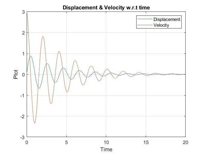
• Now , We have to take the initial condition for angular displacement and velocity for the simple pendulum.Here , the angular displacement is 0 & angular velocity is 3.
• Next the time span is defined for the following program of simple pendulum from 0 to 20 sec having 500 values in between using the linspace command.
• We can solve the second order ode by using ode45 solver which compares the method of orders four and five to estimate error and determine step size.It is so accurate that its default behavior is to use its interpolant to provide results at intermediate points.
• The syntax for the ode45 command in this matlab program is represented as [t,results]= ode45(@(t,theta) ode_function(t,theta,b,g,l,m),t_span,theta_0) where ode_function is a different matlab program for defining the function which is called to the main program.
• By using the plot command the plot for angular displacement and velocity with respect to time is plotted.Similary the xlabel and ylabel are provided to the plot.
• Hold on command is used to add a second line plot without deleting the existing line plot.
• Legend command is used to show the curve for displacement and velocity on the plot.
• Now for loop command is used for making an animation of the simple pendulum and defining the specified points of mass which is a ball at different locations and the ct command is used to count each and every position.
• In the for loop x0 and y0 coordinates are defined which are fixed and x1 y1 are the coordinates of the mass attached to the pendulum.
• Plotted the fixed line of pendulum to which the string is attached and then the plotted the string to which mass is attached.Now using the hold on command both the plots are plotted on the same figure.
• Now to make the movie we need to save the frames for different figures obtained by using getframe command and then the counter is incremented by +1 each time then the for loop is ended.
• Finally the animation for pendulum is created using the movie command.

ERRORS DURING PROGRAM:

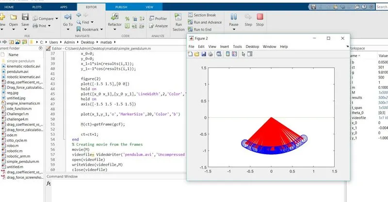
ERROR RECTIFIED:

• In the animation of simple pendulum the lines were getting printed without deleting the older line,this was because of not using the hold off command.
• Error was rectified by using hold off command.

PLOT:

LINK FOR THE ANIMATION: https://youtu.be/PIQaSnHo6t4

CONCLUSION/RESULTS:

• From the output graph obtained it can be concluded that as the time increases displacement and velocity of pendulum decreases.
• Second order ordinary differential equation for the pendulum is solved using the ode45 solver and the animation for pendulum is created.

REFERENCES:

• Figure of simple pendulum is obtained from https://byjus.com/jee/simple-pendulum/
• Animation of simple pendulum is obtained from https://commons.wikimedia.org/wiki/File:Oscillating_pendulum.gif