Project 2 - Rankine cycle Simulator

AIM: To create a Rankine cycle simulator using MATLAB.

OBJECTIVE:

1. To calculate the state points of the Rankine cycle based on user inputs.

2. To plot the corresponding T-s and h-s plots for the given set of inputs.

THEORY:

The Rankine cycle is the fundamental operating cycle of all power plants where an operating fluid is continuously evaporated and condensed. The selection of operating fluid depends mainly on the available temperature range. Figure 1 shows the idealized Rankine cycle.

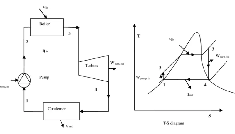
The ideal Rankine cycle does not involve any internal irreversibilities and consists of the following four processes:

1-2 isentropic compression in a pump

2-3 constant pressure heat addition in a boiler

3-4 Isentropic expansion in a turbine

4-1 constant pressure heat rejection in a condenser

water enters the pump at state 1 as saturated liquid and is compressed isentropically to the operating pressure of the boiler. The water temperature increases somewhat during this isentropic compression process due to a slight decreases in the specific volume of water.

`W_pumps = H_2-H_1`,

water enters the boiler as a compressed liquid at state 2 and leaves as a superheated vapour at state 3. The boiler is basically a large heat exchanger where the heat originating from combustion gases, nuclear reactors, or other sources is transferred to the water essentially at constant pressure. The boiler, together with the section where the steam is superheated, is ofter called the steam generator.

`Q_add = H_3-H_2`

The superheated vapor at state 3 enters the turbine, where it expands isentropically and produces work by rotating the shaft connected to an electric generator. The pressure and the generator of the steam drop during this process to the value at state 4, where steam enters the condenser. At this state, steam is usually a saturated liquid-vapor mixture with a high quality.

`W_T =H_4-H_3`

Steam is condensed at constant pressure in the condenser, which is basically a large heat exchanger, by rejecting heat to a cooling medium such as a lake, a river, or the atmosphere. steam leaves the conser as satureted liquid and enter the pumps, completing the cycle. in areas where water is precious, the power plant are cooled by air instead of water. This method of cooling , which is also used in car engines, is called dry cooling.

`Q_re = H_4-H_1`

During a Rankine cycle, work is done on the fluid by the pumps between state 1 and 2. work is done by the fluid in the turbine between stages 3 and 4. The difference between the work done by the fluid and the work done by the fluid is the net work produced by the cycle and it corresponds to the area enclosed by the cycle curve. The working fluid in a Rankine cycle follows a closed loop and is reused constantly.

As can be seen, it is convenient to use enthalpy and the first law in term of enthalpy in analysis of this thermodynamic cycle. This form of the laws simplifies the description of energy transfer. At constant pressure, the enthalpy change equals the energy transferred from the environment through heating:

Isobaric process(Vdp = 0):

dH = dQ Q = `H_2-H_1`

At constant entropy, in isentropic process, the enthalpy change equals the flow process work done on or by the system:

Isentropic process(dQ = 0)

dH = Vdp W = `H_2-H_1`

GOVERNING EQUATIONS:

• Net work done (W_NET) = W_TURBINE - W_PUMP
• Thermal efficiency (`eta`)= W_NET/Q_IN
• Work ratio(WR) = W_NET/W_TURBINE
• Back work ratio (BWR) = W_PUMP/W_TURBINE
• WR + BWR = 1,
• Heat rate (HR) = 1/`eta`
• steam rate (ssc) = 1/W_NET

BODY OF THE CONTENT:

SOLUTION STEPS:

1. To simulate and find out different state variables, all the processes parameter are to be described such as all four processes occuring and input parameters.

2. From the standard Xsteam library to get the steam table data for water, all points in between state variables are calculated. such as enthalpy, entropy, specific heat, saturation temperature, etc.

3. The calculated points are used to find out net work done, work done by turbine, thermal efficiency, back work ratio, etc according to their thermodynamic relations and necessary formulas.

4. To plot the property diagram of water, saturation liquid and vapour line , an array is created using linspace command from 0 to value of T1 with 5000 evenly spaced points in between them and suitable state variables are iterated using for loop.

5. To plot T-s and h-s diagram, all the required points are plotted and marked using text command.

MATLAB CODE:

% A program for simulating Rankine cycle plot required graphs.
close all
clear all
clc
% Subscript for different state points
% 1 = Turbine inlet or Boiler outlet, 2 = condenser inlet or Turbine
% outlet,
% 3 = Pump inlet or Condenser outlet, 4 = Boiler inlet or Pump outlet
% Input parameters-
% p1 = Turbine inlet pressure (bar),
% T1 = Temperature at turbine inlet(deg C),
% p2 = Turbine outlet pressure (bar),
% Description about four process,
fprintf('Process (1-2) - Isentropic Expansion in the Turbinen');
fprintf('Process (2-3) - Isobaric Heat Rejection by the Condensern')
fprintf('Process (3-2) - Isentropic Compression in the Pumpn')
fprintf('Process (4-1) - Isobaric Heat Addition by the Boilern')
% For Inputting state variables at point 1,
p1 = input('Enter the Pressure at the Turbine Inlet (in bar):');
T1 = input('Enter the Temperature at the Turbine inlet (in Degree celcius):');
p2 = input('Enter the pressure at the Turbine outlet (in bar):');
% Calculating state variables at all points from given datafile,
% At point 1
hg_1=XSteam('hV_p',p1);
sg_1=XSteam('sV_p',p1);
Tsat_P1=XSteam('Tsat_p',p1);
Cp1_L=XSteam('CpL_p',p1);
% At point 2
hg_2=XSteam('hV_p',p2);
sg_2=XSteam('sV_p',p2);
Tsat_p2=XSteam('Tsat_p',p2);
Cp2_V=XSteam('CpV_p',p2);
% At point 3
hf_3=XSteam('hL_p',p2);
sf_3=XSteam('sL_p',p2);
% At point 4
hf_4=XSteam('hL_p',p1);
sf_4=XSteam('sL_p',p1);
% state variables at point 1,
fprintf('At State 1n');
fprintf('p1 is :%f barn',p1);
fprintf('T1 is :%f degrees Cn',T1);
h1=XSteam('h_pt',p1,T1);
fprintf('h1 is :%f kj/kgn',h1);
s1=XSteam('s_pT',p1,T1);
fprintf('s1 is :%f kj/kgkn',s1);
% state variables at point 2,
fprintf('At State 2n');
fprintf('p2 is : %f barn', p2);
% entropy remains the same through turbine ( ideal )
s2 = s1;
fprintf('s2 is : %f kj/lgkn',s2);
% Calculating value of x(dryness fraction)
if(s2 <= sg_2)
x2 = (s2 - sf_3)/(sg_2-sf_3);
else
x2=1;
end
fprintf('x2 is :%f n',x2);
% For calculating value of T2,
if(x2<1)
T2 = Tsat_P2;
else
% s2 = sg_2 + Cp2_V*(log(T2/Tsat_P2))-formula for calculating entropy
% in superheated region
T2 = (Tsat_P2+273.15)*exp((s2-sg_2)/Cp2_V);
T2 = T2 - 273.15;
end
fprintf('T2 is : %f degrees Cn',T2)
% For calculating value of h2,
if(x2<1)
h2 = hf_3 + x2*(hg_2-hf_3);
else
h2 = XSteam('h_pT',p2,T2);
end
fprintf('h2 is : %f kj/kgn',h2)
% state variables at point 3,
fprintf('At state 3n')
p3 = p2;
fprintf('p3 is : %f barn',p3)
V3 = XSteam('vL_p',p3);
T3 = Tsat_P2;
fprintf('T3 is : %f degree Cn', T3)
h3 = hf_3;
fprintf('h3 is : %f kj/kgn',h3)
s3 = sf_3;
fprintf('s3 is : %f kj/kgn',s3)
% Calculating state variables at point 4,
fprintf('At state 4n')
p4 = p1;
fprintf('p4 is : %f barn', p4)
% Isentropic pumping process
s4 = s3;
fprintf('s4 is : %f kj/kgkn',s4)
T4 = XSteam('T_ps' ,p4,s4);
fprintf('T4 is : %f degrees Cn', T4)
W_p = V3 * (p4-p3) * 100;
h4 = W_p + h3;
fprintf('h4 is : %f kj/kgn', h4)
% Calculating of net work output, net heat, back work ratio and thermal
% efficiency and other parameters
% Work done by turbine
W_T = h1 - h2;
fprintf('Work by turbine is : %f KJ/kgn', W_T)
fprintf('Work by pump is : %f KJ/kgn', W_p)
% Net work done
Wnet = W_T - W_p;
fprintf('Net Work done is : %f KJ/kgn', Wnet)
% Net heat supplied
Qin = h1 - h4;
% Thermal Efficiency
eff_thermal = Wnet/Qin ;
fprintf('Thermal efficiency is : %fn', eff_thermal);
% Back work ratio
b_w_r = (W_p/W_T);
fprintf('Back work ratio is : %f n', b_w_r)
% Work ratio
w_r = (Wnet/W_T);
fprintf('Work ratio is : %f n', w_r)
% summation of b_w_r and w_r should be 1
fprintf('Back work ratio + work ratio is : %f n', (b_w_r+w_r))
% Heat rate and specific steam consumption
H_R = (1/eff_thermal);
fprintf('Heat Rate is : %f KJ/kwsn',H_R)
ssc = (1/Wnet);
fprintf('Specific steam consumption is : %f kg/kwsn',ssc)
% Iterating saturation Liquid and vapour linesfrom 0 to value of T1 for
% plotting property diagram of water
temperature = linspace(0, T1, 5000);
for i = 1: length(temperature)
H_l(i) = XSteam('hL_T',temperature(i));
H_v(i) = XSteam('hV_T',temperature(i));
S_l(i) = XSteam('sL_T',temperature(i));
S_v(i) = Xsteam('sV_T',temperature(i));
end
% Plotting T-s Diagram
figure(1)
hold on
plot([s1 s2],[T1 T2],'color','blue','linewidth',3)
plot([s2 sg_2],[T2 Tsat_P2],'color','green','linewidth',3)
plot([sg_2 s3],[Tsat_P2 T3],'color','green','linewidth',3)
plot([s3 s4],[T3 T4],'color','blue','linewidth',3)
plot([s4 sf_4],[T4 Tsat_P1],'color','blue','linewidth',3)
plot([sf_4 sg_1],[Tsat_P1 Tsat_P1],'color','green','linewidth',3)
plot([sg_1 s1],[Tsat_P1 T1],'color','green','linewidth',3)
text(s1,T1,' 1','FontSize',15)
text(s2,T2,' 2','FontSize',15)
text(s3,T3,' 3','FontSize',15)
text(sf_4,Tsat_P1,' 4','FontSize',15)
plot(S_1, temperature,'black','linestyle','--','linewidth', 1)
plot(S_v, temperature,'black','linestyle','--','linewidth', 1)
axis([0 10 0 500])
title('T-s Diagram of Ideal Rankine Cycle')
ylabel('Temperature (degrees C)')
xlabel('Specific Entropy (kj/kgk)')
grid on
% Plotting h-s Diagram
figure(2)
hold on
plot([s1 s2],[h1 h2],'color','green','linewidth',3)
plot([s2 sg_2],[h2 hg_2],'color','red','linewidth',3)
plot([sg_2 s3],[hg_2 h3],'color','red','linewidth',3)
plot([s3 s4],[h3 h4],'color','green','linewidth',3)
plot([s4 sf_4],[h4 hf_4],'color','green','linewidth',3)
plot([sf_4 sg_1],[hf_4 hg_1],'color','red','linewidth',3)
plot([sg_1 s1],[hg_1 h1],'color','red','linewidth',3)
text(s1,h1,' 1','FontSize',15)
text(s2,h2,' 2','FontSize',15)
text(s3,h3,' 3','FontSize',15)
text(sf_4,hf_4,' 4','FontSize',15)
plot(S_1, H_l,'color','black','linestyle','--','linewidth', 1)
plot(S_v,H_v,'color','black','linestyle','--','linewidth', 1)
title('h-s Diagram of Ideal Rankine Cycle')
ylabel('Specific Enthalpy (kj/kg)')
xlabel('Specific Entropy (kj/kgk)')
grid on

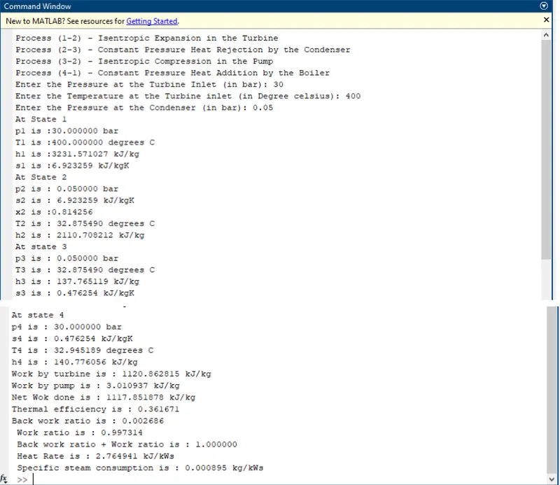
RESULTS: The following are the output of the above code-

• First user will input inlet pressure(p1), turbine inlet temperature(T1), outlet pressure(p2) and accordingly all the results will be calculated.
• For this case, the values of p1,p2,T1, are 30 bar, 0.05 bar and 400 degrees c respectively.
• The output obtained in command window is-

• The plots for T-s and h-s diagrams are as follows-

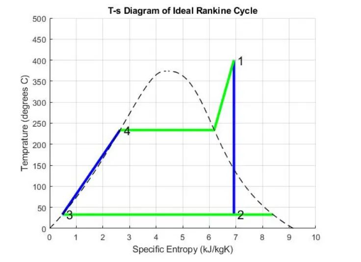
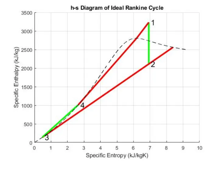
CONCLUSION:

Various programs to compute property values of water at three regions have been developed using MATLAB. Those programs are then used by another program that can simulate a Rankine cycle. This program should be useful for lecturers for the teaching of Rankine cycle as a part of thermodynamics subject. Students can also benefit from the program as well.