Week 3 - Solving second order ODEs

AIM: To simulate the transient behaviour of a simple pendulum and to create an animation of its motion on MATLAB.

OBJECTIVE:

• To write a program that solves the second order ODE corresponding to motion of a simple pendulum and to plot its angular displacement and angular velocity wrt time.
• To create the animation of the motion of pendulum.

THEORY: A simple pendulum is defined to have an object that has a small mass, also known as the pendulum bob, which is suspended from a light wire or string, such as shown in fig 1.

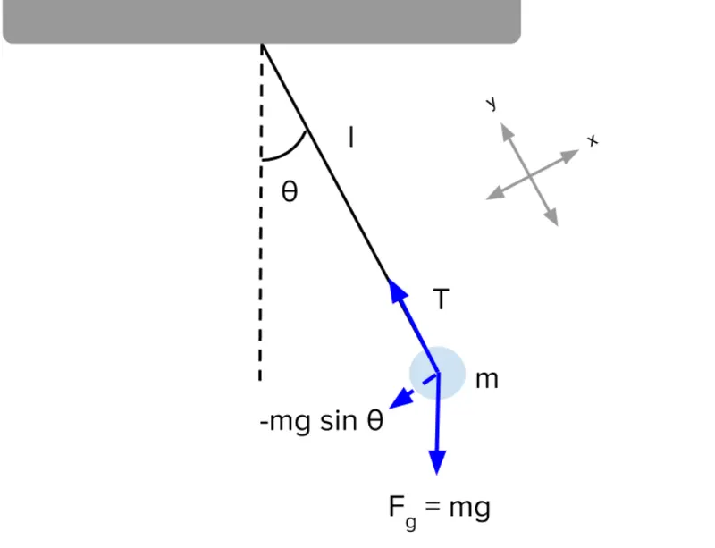
Fig 1 when the bob of pendulum is displaced from its mean position to either extreme position and is released, the pendulum will swing back and fourth with periodic motion until the motion damps. By applying newtons second law for rotational systems, the equation of motion for the pendulum may be obtained as

T= I.`alpha`

-mg.`sintheta`.L = `mL^2.d^2theta/dt^2`

and rearranged as `d^2theta/dt^2 +(g/L).sintheta`= 0

and if a damper is introduced in the system the above equation changes slightly as

`d^2theta/dt^2+(b/m).(d(theta)/dt)+(g/L).sintheta` = 0

GOVERNING EQUATIONS:

To solve the above equation in MATLAB, we need to transform the given second order ODE into first order ODE as,

`theta=theta1`,

`d(theta)/dt=d(theta1)/dt=theta2`,

`d^2theta/dt=d^2theta1/dt=d(theta2)/dt`,

`d^2theta/dt+(b/m).d(theta)/dt+(g/L).sintheta=0`,

`d^2theta1/dt+(b/m).d(theta1)/dt+(g/L).sintheta1`= 0,

`d(theta2)/dt+(b/m).theta2+(g/L).sintheta1`,

`,d(theta1)/dt=theta2`and `d(theta2)/dt=-(b/m).theta1-(g/L).sintheta1`

Represent them in matrix form which is used in MATLAB,

`d/dx[theta1 /theta2]=[theta2/-(b/m).theta2-(g/L).sintheta1]`,

BODY OF THE CONTENT:

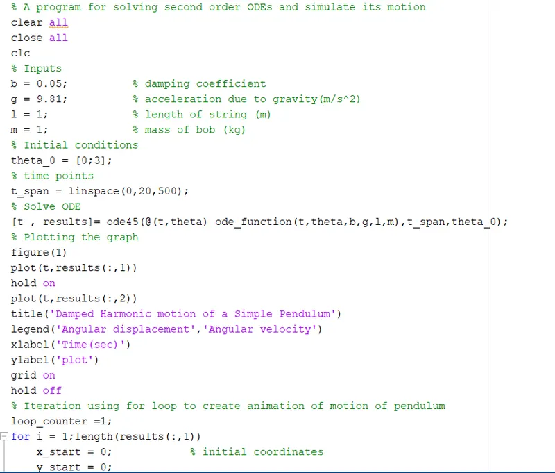
• Initial inputs such as b,g,l,m are provided according to data in the question.
• An array of initial theta was created to define initial angular displacement and initial angular velocity.
• An array of time span was created to store 500 equally spaced interval between time 0 to 20 sec.
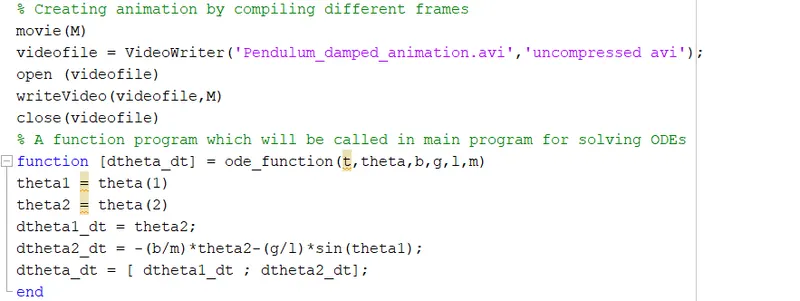
• To solve the second order ODE, a function named ode_function which store the above matrix data in it.
• The given second order ODE was solved using ode command followed by proper syntax of the calling function ode_ function and the result obtained was used to plot the graph of variation of angular displacement and angular velocity wrt time.
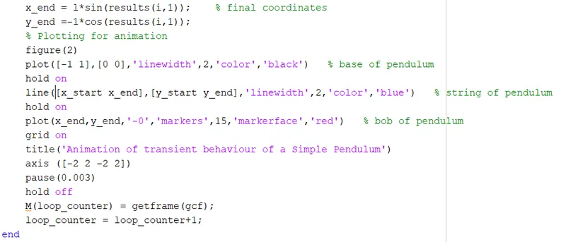
• Now for creating the animation of obtained harmonic motion of pendulum, for loop was used a loop counter variable was initiated.In this execution the one end of the string of pendulum was fixed and the other end move accordingly to the solution of the ODE solve and bob was made by using marker command and was plotted foe each time interval of the time span.
• All the frame were compiled using getframe command and movie command was used to create the animations.

MATLAB CODE FOR SOLVING AND SIMULATION:

MATLAB CODE FOR FUNCTION USED:

RESULTS:

• The following plot was generated.

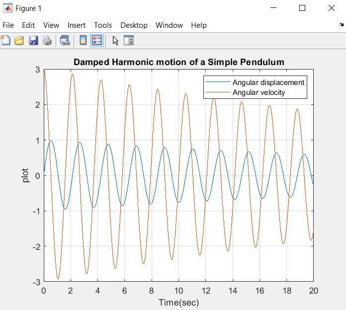
• The above plot of angular displacement and angular velocity shows the pendulum motion to be gradually decreasing. This is due to damping effect which exponentially decreases the amplitude and the velocity of motion.

CONCLUSION: In this way we can understand that any sewcond order or any higher order ODE can easily be solved using MATLAB, and simulation of transient behaviour of simple pendulum was made using it to explain the effect of damping on its motion.

REFERENCES:

b= damping coefficient(N.s/m),

g= acceleration due to gravity(m/s^2),

l= length of string(m),

m= mass of bob(kg),

`theta`= angular displacement(position)

T= torque(n.m)

I= moment of inertia(kg/m^2)

`alpha`= angular acceleration(rad/s^2)