Project 2 - Rankine cycle Simulator
- Rankine Cycle simulator
- Code to calculate state points & plot T -S & H - S Diagram
close all
clear all
clc

% Process involved in rankine cycle
disp('Rankine Cycle Simulator')
disp('1-2 : Isentropic Expansion in Turbine\n')
disp('2-3 : Constant Pressure heat rejection in condenser\n')
disp('3-4 : inentropic Compression in Water pump\n')
disp('4-1 : Constant Pressure Heat addition in Boiler\n')
disp(' ')

% Input parameters
p1 = input('Presure at turbine inlet (in Bar):');
p2 = input('Presure at turbine outlet (in Bar):');
t1 = input('Temperature at turbine inlet (in deg celcius):');
disp(' ')

% Specific heat capacity for vapour
high_cpv = XSteam('CpV_p',p1);
low_cpv = XSteam('CpV_p',p2);
high_cvv = XSteam('CvV_p',p1);
low_cvv = XSteam('CvV_p',p2);

% Specific heat capacity for liquid
high_cpL = XSteam('CpL_p',p1);
low_cpL = XSteam('CpL_p',p2);
high_cvL = XSteam('CvL_p',p1);
low_cvL = XSteam('CvL_p',p2);

% Calculation of State points

% State Points 1 Turbine Inlet & Boiler Outlet

% Enthalpy at turbine inlet
h1 = XSteam('h_pt',p1,t1);
% Entropy at turbine inlet
s1 = XSteam('s_pt',p1,t1);
% Saturated Liquid Enthalpy
hl1 = XSteam('hL_p',p1);
% Saturated Vapour Enthalpy
hg1 = XSteam('hV_p',p1);
% Saturated Liquid Entropy
sl1 = XSteam('sL_p',p1);
% Saturated Gas Entropy
sg1 = XSteam('sV_p',p1);
% Saturation Temperature
tsat1 = XSteam('Tsat_p',p1);

disp('At State point 1')
fprintf('p1 is : %f Bar\n', p1)
fprintf('t1 is : %f Deg Celcius\n', t1)
fprintf('h1 is : %f kj/kg\n', h1)
fprintf('s1 is : %f kj/kgk\n\n', s1)

% State Points 2 Turbine outlet & Condenser inlet as per state point 1

s2 = s1;% Isnetropic expansion
sl2 = XSteam('sL_p',p2);
sg2 = XSteam('sV_p',p2);
x = (s2 - sl2)/(sg2 - sl2); % Dryness factor
hl2 = XSteam('hL_p',p2);
hg2 = XSteam('hV_p',p2);
h2 = (hl2) + (x*(hg2 - hl2));
t2 = XSteam('T_ph',p2,h2);
tsat2 = XSteam('Tsat_p',p2);

disp('At State point 2')
fprintf('p2 is : %f Bar\n', p2)
fprintf('t2 is : %f Deg Celcius\n', t2)
fprintf('h2 is : %f kj/kg\n', h2)
fprintf('s2 is : %f kj/kgk\n\n', s2)

% state Points 3 Condenser outlet & Pump Inlet
t3 = tsat2; % phase change from vapour to liquid
p3 = p2; % Constant pressure heat rejection
s3 = sl2;
h3 = hl2;
v3 = XSteam('vL_p',p3);

disp('At State point 3')
fprintf('p is : %f Bar\n', p3)
fprintf('t3 is : %f Deg Celcius\n', t3)
fprintf('h3 is : %f kj/kg\n', h3)
fprintf('s3 is : %f kj/kgk\n\n', s3)

% state point 4 pump outlet & boiler inlet
p4 = p1; % Constant presure heat addition
s4 = s3;% Isentropic compression
Wp = v3*(p4 - p3)*100;
h4 = Wp + h3;
l = exp((sl1-s4)/high_cpL);
t4 = tsat1/l;
disp('At State point 4')
fprintf('p4 is : %f Bar\n', p4)
fprintf('t4 is : %f Deg Celcius\n', t4)
fprintf('h4 is : %f kj/kg\n', h4)
fprintf('s4 is : %f kj/kgk\n\n', s4)

% Work done by turbine Wt
Wt = h1 - h2;
disp(' Work done by turbine')
fprintf(' Work done by Turbine is : %f kj/kgk\n\n', Wt)

% Work Done by pump
Wp = v3*(p4 - p3)*100;
disp(' Work done by Pump')
fprintf(' Work done by Pump is : %f kj/kgk\n\n', Wp)

% Nett work done
Wn = Wt - Wp;
disp(' Nett Work done')
fprintf(' Nett work done is : %f kj/kgk\n\n', Wn)
Qin = h1 - h4;

% Thermal efficiency of cycle
Eth = Wn/Qin ;
disp(' Thermal efficiency of cycle')
fprintf(' Thermal efficiency of cycle is : %f', Eth*100); disp('%')
fprintf('\n')

% Specific steam consumption
ssc = 3600 / Wt;
disp(' Specific steam consumption')
fprintf(' Specific steam consumption : %f kg/kwh\n\n', ssc)

% Plotting

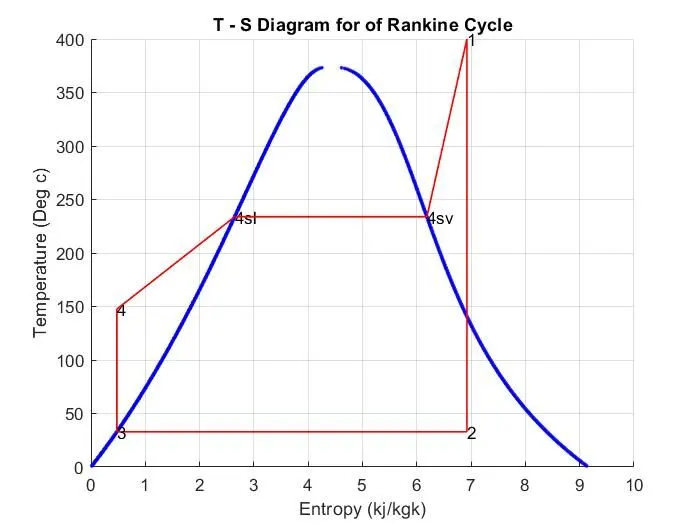
% T - S Diagram
figure(1), clf
hold on

% Saturation Curve
t = linspace(1,373.15,500);
for i = 1:length(t)
    plot(XSteam('sL_T',t(i)),t(i), 'b.','linestyle','--','linewidth',1)
    plot(XSteam('sV_T',t(i)),t(i), 'b.','linestyle','--','linewidth',1)
end
% Rankine Cycle
plot([s1 s2],[t1 t2],'r','linewidth',1)
text(s1,t1,'1')
text(s2,t2,'2')
plot([s2 s3],[t2 t3],'r','linewidth',1)
text(s3,t3,'3')
plot([s3 s4],[t3 t4],'r','linewidth',1)
text(s4,t4,'4')
plot([s4 sl1],[t4 tsat1],'r','linewidth',1)
text(sl1,tsat1,'4sl')
plot([sl1 sg1],[tsat1 tsat1],'r','linewidth',1)
text(sg1,tsat1,'4sv')
plot([sg1 s1],[tsat1 t1],'r','linewidth',1)
title('T - S Diagram for of Rankine Cycle')
ylabel('Temperature (Deg c)')
xlabel('Entropy (kj/kgk)')
grid on


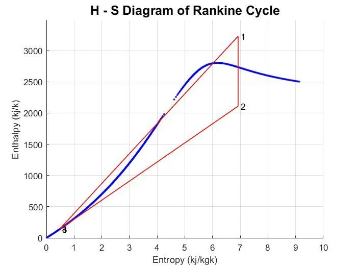
figure(2)
hold on
% Saturation Curve
for i = 1:length(t)
    plot(XSteam('sL_T',t(i)),XSteam('hL_T',t(i)), 'b.','linestyle','--','linewidth',1)
    plot(XSteam('sV_T',t(i)),XSteam('hV_T',t(i)), 'b.','linestyle','--','linewidth',1)
end
% Rankine Cycle
plot([s1 s2],[h1 h2],'r','linewidth',1)
text(s1,h1,' 1')
plot([s2 s3],[h2 h3],'r','linewidth',1)
text(s2,h2,' 2')
plot([s3 s4],[h3 h4],'r','linewidth',1)
text(s3,h3,' 3')
plot([s4 s1],[h4 h1],'r','linewidth',1)
text(s4,h4,' 4')
title('H - S Diagram of Rankine Cycle','Fontsize',15)
ylabel('Enthalpy (kj/k)')
xlabel('Entropy (kj/kgk)')
grid on
- Results
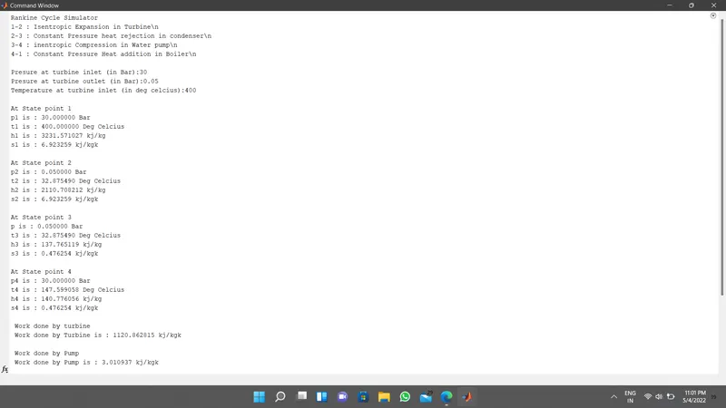
1. Command Window
Rankine Cycle Simulator
1-2 : Isentropic Expansion in Turbine\n
2-3 : Constant Pressure heat rejection in condenser\n
3-4 : inentropic Compression in Water pump\n
4-1 : Constant Pressure Heat addition in Boiler\n
Presure at turbine inlet (in Bar):30
Presure at turbine outlet (in Bar):0.05
Temperature at turbine inlet (in deg celcius):400
At State point 1
p1 is : 30.000000 Bar
t1 is : 400.000000 Deg Celcius
h1 is : 3231.571027 kj/kg
s1 is : 6.923259 kj/kgk
At State point 2
p2 is : 0.050000 Bar
t2 is : 32.875490 Deg Celcius
h2 is : 2110.708212 kj/kg
s2 is : 6.923259 kj/kgk
At State point 3
p is : 0.050000 Bar
t3 is : 32.875490 Deg Celcius
h3 is : 137.765119 kj/kg
s3 is : 0.476254 kj/kgk
At State point 4
p4 is : 30.000000 Bar
t4 is : 147.599058 Deg Celcius
h4 is : 140.776056 kj/kg
s4 is : 0.476254 kj/kgk
Work done by turbine
Work done by Turbine is : 1120.862815 kj/kgk
Work done by Pump
Work done by Pump is : 3.010937 kj/kgk
Nett Work done
Nett work done is : 1117.851878 kj/kgk
Thermal efficiency of cycle
Thermal efficiency of cycle is : 36.167131%
Specific steam consumption
Specific steam consumption : 3.211811 kg/kwh
2. T - S Diagram
2. H - S Diagram
3. Command Window
- Report
1. Understanding thermodynamic processes
2. understanding the rankine cycle with
- Thermodynamic processes involved
- Relations of termodynamic processes among temp, pressure, volume, entapy,entrpy
- T - S Diagram
- H - S Diagram
- Saturation Curve
3. Data Extraction formats from steam table
4. understand and display the processes involved in rankine cycle
disp('Rankine Cycle Simulator')
disp('1-2 : Isentropic Expansion in Turbine\n')
disp('2-3 : Constant Pressure heat rejection in condenser\n')
disp('3-4 : inentropic Compression in Water pump\n')
disp('4-1 : Constant Pressure Heat addition in Boiler\n')
disp(' ')
5. Receives user input for stage 1
p1 = input('Presure at turbine inlet (in Bar):');
p2 = input('Presure at turbine outlet (in Bar):');
t1 = input('Temperature at turbine inlet (in deg celcius):');
disp(' ')
6. Extract Cpecific heat data from XSteam for vapour stage
high_cpv = XSteam('CpV_p',p1);
low_cpv = XSteam('CpV_p',p2);
high_cvv = XSteam('CvV_p',p1);
low_cvv = XSteam('CvV_p',p2);
7. Extract Cpecific heat data from XSteam for liquid stage
high_cpL = XSteam('CpL_p',p1);
low_cpL = XSteam('CpL_p',p2);
high_cvL = XSteam('CvL_p',p1);
low_cvL = XSteam('CvL_p',p2);
8. Calculation for state points
1. State Points 1 Turbine Inlet & Boiler Outlet
Enthalpy at turbine inlet
Enthalpy at pressure p1 & temperature t1
h1 = XSteam('h_pt',p1,t1);
Entropy at turbine inlet
Enthalpy at pressure p1 & temperature t1
s1 = XSteam('s_pt',p1,t1);
Saturated Liquid Enthalpy at pressure p1
hl1 = XSteam('hL_p',p1);
Saturated Vapour Enthalpy at pressure p1
hg1 = XSteam('hV_p',p1);
Saturated Liquid Entropy at pressure p1
sl1 = XSteam('sL_p',p1)
Saturated Gas Entropy at pressure p1
sg1 = XSteam('sV_p',p1);
Saturation Temperature at pressure p1
tsat1 = XSteam('Tsat_p',p1);
Dispaly State point 1 Variables
disp('At State point 1')
fprintf('p1 is : %f Bar\n', p1)
fprintf('t1 is : %f Deg Celcius\n', t1)
fprintf('h1 is : %f kj/kg\n', h1)
fprintf('s1 is : %f kj/kgk\n\n', s1)
2. State Points 2 Turbine outlet & Condenser inlet as per state point 1
As processed in stage 1 calculated state points for stage 2 with help of thermodynamic relations for thermodynamic processes & XSteam File
s2 = s1; Isnetropic expansion
sl2 = XSteam('sL_p',p2);
sg2 = XSteam('sV_p',p2);
x = (s2 - sl2)/(sg2 - sl2); Dryness factor
hl2 = XSteam('hL_p',p2);
hg2 = XSteam('hV_p',p2);
h2 = (hl2) + (x*(hg2 - hl2));
t2 = XSteam('T_ph',p2,h2);
tsat2 = XSteam('Tsat_p',p2);
Dispaly State point 2 Variables
disp('At State point 2')
fprintf('p2 is : %f Bar\n', p2)
fprintf('t2 is : %f Deg Celcius\n', t2)
fprintf('h2 is : %f kj/kgn', h2)
fprintf('s2 is : %f kj/kgk\n\n', s2)
3. state Points 3 Condenser outlet & Pump Inlet
As processed in stage 2 calculated state points for stage 2 with help of thermodynamic relations for thermodynamic processes & XSteam File
t3 = tsat2; phase change from vapour to liquid
p3 = p2; Constant pressure heat rejection
s3 = sl2; liquid stage at state 3
h3 = hl2; liquid stage at state 3
v3 = XSteam('vL_p',p3); liquid stage at state 3
Dispaly State point 3 Variables
disp('At State point 3')
fprintf('p is : %f Bar\n', p3)
fprintf('t3 is : %f Deg Celcius\n', t3)
fprintf('h3 is : %f kj/kg\n', h3)
fprintf('s3 is : %f kj/kgk\n\n', s3)
4. state point 4 pump outlet & boiler inlet
p4 = p1; Constant presure heat addition
s4 = s3; Isentropic compression
Wp = v3*(p4 - p3)*100; Work done by pump
h4 = Wp + h3; enthalpy after compression = work done by compressor + Entalpy at stage 3
l = exp((sl1-s4)/high_cpL);
t4 = tsat1/l;
Display State point 4
disp('At State point 4')
fprintf('p4 is : %f Bar\n', p4)
fprintf('t4 is : %f Deg Celcius\n', t4)
fprintf('h4 is : %f kj/kg\n', h4)
fprintf('s4 is : %f kj/kgk\n\n', s4)
- Performance parameters of Rankine Cycle
Work done by turbine Wt
Wt = h1 - h2;
disp(' Work done by turbine')
fprintf(' Work done by Turbine is : %f kj/kgk\n\n', Wt)
ork Done by pump
Wp = v3*(p4 - p3)*100;
disp(' Work done by Pump')
fprintf(' Work done by Pump is : %f kj/kgk\n\n', Wp)
Nett work done
Wn = Wt - Wp;
disp(' Nett Work done')
fprintf(' Nett work done is : %f kj/kgk\n\n', Wn)
Qin = h1 - h4;
Thermal efficiency of cycle
Eth = Wn/Qin ;
disp(' Thermal efficiency of cycle')
fprintf(' Thermal efficiency of cycle is : %f', Eth*100); disp('%')
fprintf('\n')
Specific steam consumption
ssc = 3600 / Wt;
disp(' Specific steam consumption')
fprintf(' Specific steam consumption : %f kg/kwh\n\n', ssc)
9. Plot Saturation curve
using linspace divide temperature range 0 to 100 deg celcius in kelvin
for twmperature range of linspace plot a graph pf saturation curve against liquid entropy & Vapour Entropy at each temperature value of linspace
10 . With the help of state points calculated plot the graph for T S Diagram & H S Diagram along with saturation Curve