Project 2 - Rankine cycle Simulator

AIM:

• To simulate a Rankine cycle using matlab.
• Extracting steam and water properties from Xstram file.
• Calculating all the state points of the cycle based on user inputs.
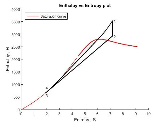
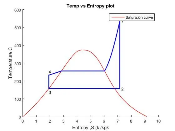
• Plotting thet T vs S and H vs S plot the given input.

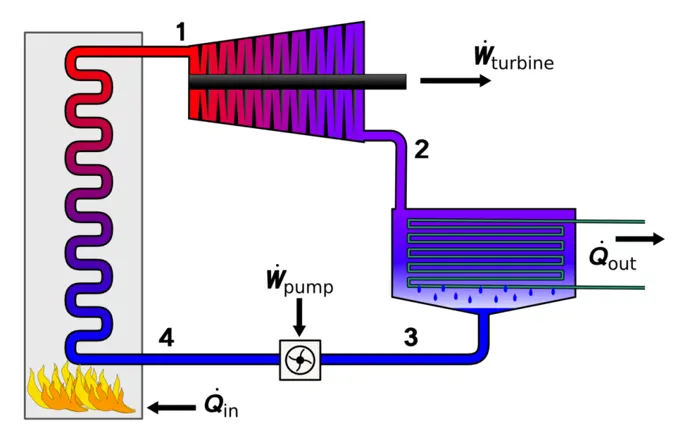
Theory - A rankine cycle is an idealised Thermodynamic cycle which governs the working of a Heat Engine.In Ranking cycle,the friction losses of a heat engine are neglected. It is a cycle which converts heat into mechanical energy which usually is converted into electrical energy.There are four componenets are Turbine,Condensor,Pump and Boiler.Rankine cycle is nothing but a modification of Carnot cycle Ideal Rankine cycle is very useful in steam power plants and gas power plants.To improve the efficiency of Rankine cycle in the steam power plants.To improve the efficiency of Rankine cycle in the steam power plant,There are some changes in Rankin cycle which differs from Carnot cycle .Firstly a pump is used in place of condenser to handle only liquid, not a mixture of liquid and vapour.Secondly exhaust steam from the turbine is completely condensed int the condenser, see in the following diagram:

Processes and working:

There are four process in the rankine cycle:

1. Process 1-2 : Isentropic Expansion in the turbine

2. Process 2 -3 : Constant Pressure heat rejection in the condenser

3. Process 3 - 4 : Isentropic Compression in the pump

4. Process 4 - 1 : Constant Pressure heat addition in the boiler

• Process 1-2 the dry saturatd vapour expands through a turbine, generating power.This decrease the temperature and presure of the vapour and some condensation may occure.
• Process 2-3 the vapour liquid mixyure leaving the turbine is condensed at low pressure usually in a surface condenser using cooling water .In well designed and maintained condensers the pressure of the vapour is well below atmosheric pressure,approaching the saturation pressure of the operating fluid at the cooling temperature.
• Process 3-4 the pressure of the condensate is raised in the feed pump.because of the low specific volume of liquids the pump work is relatively small and often neglected in thermodynamic calculations.
• Process 4-1 high pressure liquid enters the boiler from the feed pump and is heated (to the saturation temperature on the saturation curve).Further addition of energy causes evaporation of the liquid until it is fully converted to saturated steam or superheated.

Back Work Ratio:

The fraction of the work produced by the turbine that is consumed by the compressor.

BW ratio = Wp/Wt

Explanation of Program :

• Xsteam data is used to xtract steam and water properties of enthalpy , entropy at specific pressure and temperatures for sat liquid,sat vapour conditions etc.
• The program requires the input of pressure (in bar)at state point 1 (turbine inlet),Temperature at same point(degree celcius) and pressure at condenser inlet (point 2).
• with the help of these inlets & from xsteam data,the program calculates all the state points of the Rankine cycle.
• The xsteam data works as h1=Xsteam('h_pT',p1,T1) it returns the enthalpy of water at given pressure and temperature in bar and degree respectively.
• As we extract the data, we use thermodynamic relation to further find state points and extract their data from xsteam which are mentioned after studying the rankine cycle.
• Sf and Sg , Hf and Hg where f and g stands for satured liquid and saturated vapour respectively are calculated after studying the plots of Rankine cycles and extracting data from xsteam file.
• The net woek, work done by turbine , work done to run the pumpheat in and heat out are calculated using standard thermodynamic relation.
• Efficiency and specific steam consumptions of the Rankine cycle is calculated form thermodynamic relation and mentioning them in program using relations.
• T,S and H are extracted at vapour and liquid line for plotting purpose,after 4th point for the variation you observe in the plot
• Saturation curve is plotted in red for saturated liquid and saturated gas in T-S and H-S it is back.
• Plot of T vs S and H vs S is created from all the points obtained from the program using plot command and mentioning the labels,linewidth,color and tiltle.
• The plot changes as the user input changes for above mentioned inputs.
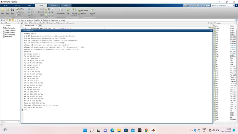
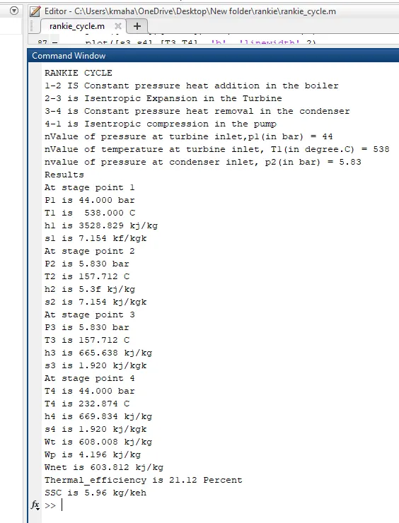
• Results are displayed in the command window by using sprint command.

Main code:

clear all
close all
clc
disp('RANKIE CYCLE')
disp('1-2 IS Constant pressure heat addition in the boiler')
disp('2-3 is Isentropic Expansion in the Turbine')
disp('3-4 is Constant pressure heat removal in the condenser')
disp('4-1 is Isentropic compression in the pump');

%obtaining the input data

p1 = input('nValue of pressure at turbine inlet,p1(in bar) = ');
T1 = input('nValue of temperature at turbine inlet, T1(in degree.C) = ');
p2 = input('nvalue of pressure at condenser inlet, p2(in bar) = ');

% At state 1
h1 = Xsteam('h_pt' , p1, T1);
s1 = Xsteam('s_pt' , p1, T1);
%At state 2
s2 = s1;
sf2 = Xsteam('sL_p',p2);
sg2 = Xsteam('sV_p',p2);
x2 = (s2 - sf2)/(sg2 - sf2);
hf2 = Xsteam('hL_p',p2);
hg2 = Xsteam('hV_p',p2);
h2 = hf2 + (x2*(hg2-hf2));

% At state 3
p3 = p2;
s3 = Xsteam('sL_P' , p3);
h3 = Xsteam('hL_p' , p3);

% At state 4
s4 = s3;
p4 = p1;
% Work done by turbine;
Wt = h1 - h2;

%work done to run pump
v3 = Xsteam('vL_p',p3);
Wp = v3*(p4 - p3)*100;
h4 = h3 + Wp;
%Net work
Wnet = Wt - Wp;
%Heat into the system
Qin = h1 - h4;
% Heat out of the system
Qout = h2 - h3;
%Thermal efficiency
thermal_eff = (Wnet/Qin)*100;
%specific steam consumption
%SSC = mass flow rate/power
SSC = (3600/Wnet);

% Calculation of Temperture at the state points
T3 = Xsteam('Tsat_p', p3);
T2 = T3;
Cp4 = Xsteam('Cp_ps' , p4, s4);
Cv4 = Xsteam('Cv_ps' , p4, s4);
k = Cp4/Cv4;
T4 = T3/((p3/p4)^((k-1)/k));

% Calculating Temperature, Entropy and Enthalpy at the vapour and liquid
% line for plotting
T6 = Xsteam('Tsat_p' , p1);
s5 = Xsteam('sL_p' , p1);
s6 = Xsteam('sV_p' , p1);
h5 = Xsteam('hL_p' , p1);
h6 = Xsteam('hV_p' , p1);
T5 = T6;
%plotting the saturation curve
T = linspace(1,375,1000);
for i = 1:length(T)
sf(i) = Xsteam('sL_T' , T(i));
sg(i) = Xsteam('sV_T' , T(i));
hf(i) = Xsteam('hL_T' , T(i));
hg(i) = Xsteam('hV_T' , T(i));
end

%Plotting T-s diagram
figure(1)
hold on
plot(sf, T,'r','linewidth',1)
plot(sg, T, 'r','linewidth',1)
plot([s1 s2],[T1 T2], 'b', 'linewidth',2)
plot([s2 s3],[T2 T3], 'b', 'linewidth',2)
plot([s3 s4],[T3 T4], 'b', 'linewidth',2)
plot([s4 s5],[T4 T5], 'b', 'linewidth',2)
plot([s5 s6],[T5 T6], 'b', 'linewidth',2)
sc1 = linspace(s6,s1,1000);
for l = 1:length(sc1)
Tc1(l) = Xsteam('T_ps' ,p1, sc1(l));
end
plot(sc1, Tc1, 'b', 'linewidth' , 2)
text(s1+0.1, T1, '1')
text(s2+0.1, T2, '2')
text(s3, T3-20, '3')
text(s4, T4+20, '4')
title('Temp vs Entropy plot')
xlabel('Entropy ,S (kj/kgk')
ylabel('Temperature C')
legend('Saturation curve')

%plotting h-s diagram
figure(2)
hold on
plot(sf, hf, 'r', 'linewidth',1)
plot(sg, hg,'r','linewidth',2)
plot([s1 s2], [h1 h2], 'k', 'linewidth',2)
plot([s2 s3], [h2 h3], 'k', 'linewidth',2)
plot([s3 s4], [h3 h4], 'k','linewidth',2)
hc = linspace(h4 , h5, 100);
for k = 1:length(hc)
sch(k) = Xsteam('s_ph' , p1, hc(k));
end
plot(sch, hc,'k','linewidth',2)
plot([s5 s6],[h5 h6],'k','linewidth',2)
for m = 1:length(sc1)
hc1(m) = Xsteam('h_ps' ,p1,sc1(m));
end
plot(sc1,hc1,'k','linewidth',2)
text(s1+0.1,h1,'1')
text(s2+0.1, h2, '2')
text(s3, h3-100, '3')
text(s4, h4+200,'4')
title('Enthalpy vs Entropy plot')
xlabel('Entropy , S')
ylabel('Enthalpy , H')
legend('Saturation curve','location','northwest')

%Displaying the results in the command Window:
disp('Results');
p1 = p1;
T1 = T1;
p2 = p2;
disp('At stage point 1')
n1 = sprintf('P1 is %.3f bar',p1);
disp(n1);
n2 = sprintf('T1 is % .3f C',T1);
disp(n2);
n3 = sprintf('h1 is %.3f kj/kg',h1);
disp(n3);
n4 = sprintf('s1 is %.3f kf/kgk',s1);
disp(n4);
disp('At stage point 2');
n11= sprintf('P2 is %.3f bar',p2);
disp(n11);
n21 = sprintf('T2 is %.3f C',T2);
disp(n21);
n31 = sprintf('h2 is 5.3f kj/kg',h2);
disp(n31);
n41 = sprintf('s2 is %.3f kj/kgk',s2);
disp(n41);
disp('At stage point 3');
n12 = sprintf('P3 is %.3f bar' ,p3);
disp(n12);
n22 = sprintf('T3 is %.3f C' ,T3);
disp(n22);
n32 = sprintf('h3 is %.3f kj/kg',h3);
disp(n32);
n42 = sprintf('s3 is %.3f kj/kgk',s3);
disp(n42);
disp('At stage point 4');
n13 = sprintf('T4 is %.3f bar',p4);
disp(n13);
n23 = sprintf('T4 is %.3f C',T4);
disp(n23);
n33 = sprintf('h4 is %.3f kj/kg' , h4);
disp(n33);
n43 = sprintf('s4 is %.3f kj/kgk',s4);
disp(n43);
n14 = sprintf('Wt is %.3f kj/kg',Wt);
disp(n14);
n15 = sprintf('Wp is %.3f kj/kg',Wp);
disp(n15);
n16 = sprintf('Wnet is %.3f kj/kg',Wnet);
disp(n16);
n17 = sprintf('Thermal_efficiency is %.2f Percent',thermal_eff);
disp(n17);
n18 = sprintf('SSC is %.2f kg/keh',SSC);
disp(n18);