Project 2 - Rankine cycle Simulator
(Project - 2 Rankine cycle simulator)
AIM:
To create a Rankine cycle simulator by using MatLab with the help of the inbuild Xsteam library.
EQUATIONS/FORMULAE:
By using Xsteam library we can find all the 6 state variables.
Work done by the Turbine
`W_T=h_1-h_2`
Work done by the Pump
`W_P=h_4-h_3` or `W_P=V_ftimes(P_1-P_2)`
Net work done
`W_N=W_T-W_P`
Heat Addition
`Q_(IN)=h_1-h_4`
Heat Rejection
`Q_(OUT)=h_2-h_3`
Thermal Efficiency
`eta_(th)=(W_N/Q_(IN))times100`
Back Work Ratio
`BWR=W_P/W_T`
Specific steam consumption
`SSC=3600/W_N`
OBJECTIVES:
- need to calculate all the state variables by using Xsteam library.
- plot the graph of Temperature vs Entropy and Enthalpy vs Entropy.
- create a Rankine cycle simulator to do the above objectives.
BODY OF THE CONTENT:
Rankine cycle?
The Rankine cycle is an idealized thermodynamic cycle describing the process by which certain heat engines, such as steam turbines or reciprocating steam engines, allow mechanical work to be extracted from a fluid as it moves between a heat source and heat sink.
This Rankine cycle consists of 4 process
- 1-2 is Isentropic Expansion in the Turbine
- 2-3 is Const Pressure Heat Rejection by the Condenser
- 3-4 is Isentropic Compression in the Pump
- 4-1 is Const Pressure Heat Addition by the Boiler
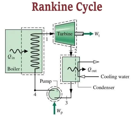
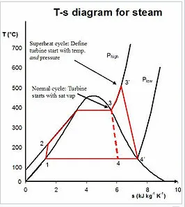
- for this calculation first, we need to find the all-state point variables with help of some required inputs. After that, we generally calculate the value and plot the graph of T-S and H-S in MatLab.
- By using the above MatLab code concept, we create it as a simulator of the Rankine cycle.
- NOTE: state point variables are found by using the steam table in MatLab which is called Xsteam.m file give the link below(which is not coded by me. It's already available)
https://drive.google.com/file/d/1RK_fvrOj38CIaQvmLT1S3daqHnxKCGU-/view
CODE:
MAIN CODE
% Rankine cycle simulator
clear,close,clc
% code to ask inputs
fprintf('%75s\n\n','RANKINE CYCLE SIMULATOR')

fprintf('1-2 is Isentropic Expansion in the Turbine\n')
fprintf('2-3 is Const Pressure Heat Rejection by the Condenser\n')
fprintf('3-4 is Isentropic Compression in the Pump\n')
fprintf('4-1 is Const Pressure Heat Addition by the Boiler\n\n')

p1 = input('Enter the pressure at the Turbine(in Bar): ');
t1 = input('Enter the temperature at the Turbine(in degree Celcius): ');
p2 = input('Enter the pressure at the condenser(in Bar) : ');
% calculation part using rankine_cycle function
[result] = rankine_cycle(t1,p1,p2);
for i = 1:6
    h(i) = result(i,1);
    s(i) = result(i,2);
    t(i) = result(i,3);
    p(i) = result(i,4);
end
W_T = result(7,1);
W_p = result(7,2);
W_n = result(7,3);
Q_in = result(7,4);
Q_out = result(8,1);
n_therm = result(8,2)*100;
BWR = result(8,3);
SSc = result(8,4);
% code for plots T-S and H-S Diagram
T = linspace(0,t1,1000);
for i = 1:length(T)
    h_L_line(i) = XSteam('hL_T',T(i));
    h_V_line(i) = XSteam('hV_T',T(i));
    s_L_line(i) = XSteam('sL_T',T(i));
    s_V_line(i) = XSteam('sV_T',T(i));
    x2 = result(9,1);
end
figure(1)
plot([s(1) s(2) s(3) s(4) s(5) s(6) s(1)],[t(1) t(2) t(3) t(4) t(5) t(6) t(1)],Color='r')
hold on
plot([s_L_line s_V_line],[T T],Color=[0 0 0])
xa = [s(1) s(2) s(3) s(4) s(5) s(6)];
ya = [t(1) t(2) t(3) t(4) t(5) t(6)];
txt = {'1','2','3','4','5','6'};
text(xa,ya,txt)
title('Rankine cycle T-S Diagram')
xlabel('Entropy(kJ/kgK)')
ylabel('Temperature(''C)')
hold off

figure(2)
plot([s(1) s(2) s(3) s(4) s(5) s(6) s(1)],[h(1) h(2) h(3) h(4) h(5) h(6) h(1)],Color='r')
hold on
plot([s_L_line s_V_line],[h_L_line h_V_line],Color=[0 0 0])
xa = [s(1) s(2) s(3) s(4) s(5) s(6)];
ya = [h(1) h(2) h(3) h(4) h(5) h(6)];
txt = {'1','2','3','4','5','6'};
text(xa,ya,txt)
title('Rankine cycle H-S Diagram')
xlabel('Entropy (kJ/kgK)')
ylabel('Enthalpy(kJ/kg)')
% showing the output in command window
fprintf('\n')
fprintf('%70s\n','RESULTS:')
for i = 1:6
    fprintf('State variables at state point (%d)\n\n',i)
    fprintf('Pressure(p%d) = %f bar\n',i,p(i))
    fprintf('Temparature(t%d) = %f ''C\n',i,t(i))
    fprintf('Enthalpy(h%d) = %f kJ/kg\n',i,h(i))
    if i~= 2
    fprintf('Entropy(s%d) = %f kJ/kgK\n\n',i,s(i))
    end
    if i == 2
        fprintf('Entropy(s%d) = %f kJ/kgK\n',i,s(i))
        fprintf('x2 = %f\n\n',result(9,1));
    end
end

fprintf('Work done by Turbine = %f kJ\n',W_T)
fprintf('Work done by Pump = %f kJ\n',W_p)
fprintf('Net work done = %f kJ\n',W_n)
fprintf('Amount of heat added = %f kJ\n',Q_in)
fprintf('Amount of heat rejected = %f kJ\n',Q_out)
fprintf('Thermal efficiency = %.2f%%\n',n_therm)
fprintf('Back work ratio = %f\n',BWR)
fprintf('Specific steam consumption = %f kg/kWh\n',SSc)
FUNCTION CODE
% code to find the state points variables
function [results] = rankine_cycle(t1,p1,p2)
% state point 1
h1 = XSteam('h_pT',p1,t1);
s1 = XSteam('s_pT',p1,t1);
% state point 2
s2 = s1;
sf2 = XSteam('sL_p',p2);
sg2 = XSteam('sV_p',p2);
sfg2 = sg2-sf2;
x2 = (s1-sf2)/sfg2;
hg2 = XSteam('hV_p',p2);
hf2 = XSteam('hL_p',p2);
hfg2 = hg2-hf2;
h2 = hf2 + x2*hfg2;
t2 = XSteam('T_ps',p2,s2) ;
% state point 3
p3 = p2;
t3 = t2;
h3 = hf2;
s3 = sf2;
spec_volumef = XSteam('vL_p',p2);
% state point 4
p4 = p1;
W_p = spec_volumef*(p4-p2)*100;
h4 = h3+W_p;
s4 = s3;
cp = XSteam('Cp_ps',p4,s4);
cv = XSteam('Cv_ps',p4,s4);
gamma = cp/cv;
t4 = t3*(p4/p3)^((gamma-1)/gamma);
% state point 5
p5 = p4;
s5 = XSteam('sL_p',p4);
h5 = XSteam('hL_p',p4);
t5 = XSteam('Tsat_p',p4);
% state point 6
p6 = p5;
s6 = XSteam('sV_p',p4);
h6 = XSteam('hV_p',p4);
t6 = t5;
% calculation
W_T = h1 - h2;
W_n = W_T - W_p;
Q_in = h1 - h4;
Q_out = h2 - h3;
n_therm = W_n/Q_in;
BWR = W_p/W_T;
SSc = 3600/W_n;

% storing all the results
results = [h1 s1 t1 p1;h2 s2 t2 p2;h3 s3 t3 p3;h4 s4 t4 p4;h5 s5 t5 p5;h6 s6 t6 p6;W_T W_p W_n Q_in;Q_out n_therm BWR SSc;x2 0 0 0];
end
EXPLANATION OF CODE:
MAIN CODE
- From code lines 1 to 2 - clear all the previous data.
- From code lines 3 to 13 - code for the output screen and ask the inputs to simulate the Rankine cycle.
- From code lines 14 to 29 - performing the Rankine cycle simulator by using the input values in the Rankine_cycle function program and saving all the extracted answers we want in different variables.
- From code lines 30 to 38 - creating the values for saturated line for T-s and H-S plots.
- From code lines 39 to 62 - code to plot T-S and H-S Diagram with proper label and title.
- From code lines 63 to 87 - code to show all the outputs in the command window.
FUNCTION CODE
- From code lines 1 to 2 - creating the function called Rankine_cycle
- From code lines 3 to 5 - finding the value of h and S of state variable 1 by using Xsteam data file.
- From code lines 6 to 16 - finding the values for state point variables 2 by using Xsteam.
- From code lines 17 to 22 - finding the state point variables of state point 2 and additionally specific volume for future use.
- From code lines 23 to 31 - finding the state point variable at state point 4 by using Xsteam.
- From code lines 32 to 36 - for state point 5.
- From code lines 37 to 41 - for state point 6.
- From code lines 42 to 49 - by using all the state point variables, we calculate the work done, heat inputs, outputs, thermal efficiency, and all the values we need are calculated.
- From code lines 51 to 53 - storing all the calculated value into a variable called results and returning to the function and end the function.
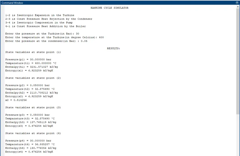
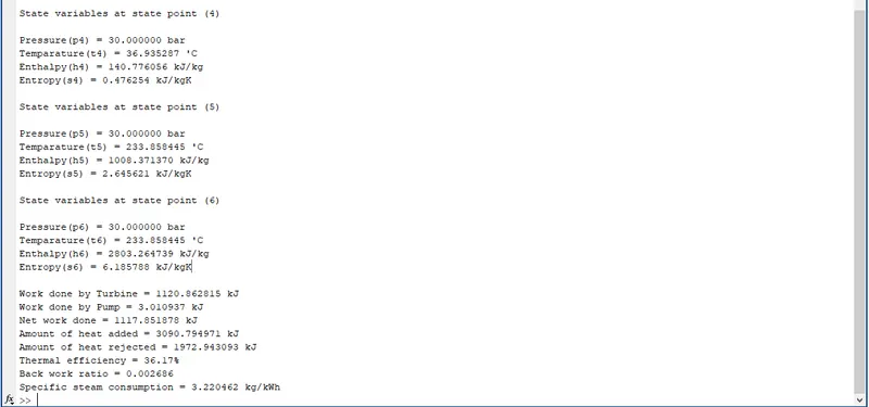
RESULTS:
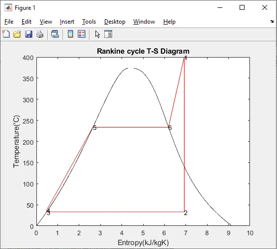
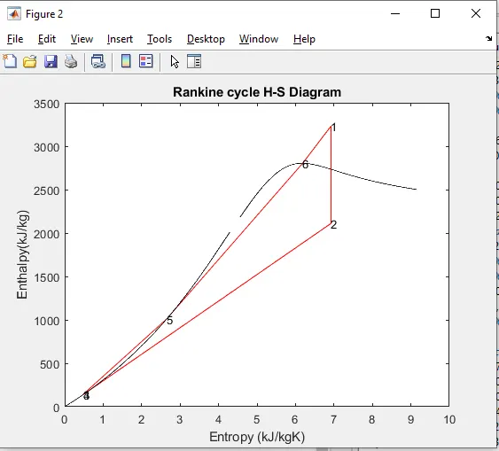
ERROR:
I faced a lot of errors with spelling mistakes and forgetting to close or open the bracket and also some other errors which are given below.
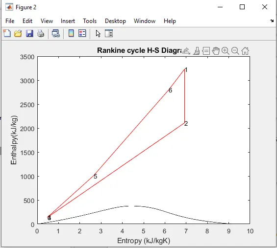
the above error is due to the wrong y coordinate inputs.

The size of the matrix is not equal that's why the above error poped up.

The above error is due to I forgot to mention the pressure.

The above error is due to I providing extra input to the text command operator accidentally.

index problem
CONCLUSION:
The Rankine cycle simulator was created successfully. Turbine input of pressure and Temperature and condenser input pressure are the inputs of this simulator. by using these inputs, This Rankine cycle simulator gives us the state point variables, heat input, heat output, work done by the Turbine and pump, and efficiency of the cycle and so on as an output.
REFERENCE: