Project 2 - Rankine cycle Simulator

AIM:

To create Rankine cycle simulator in MATLAB.

OBJECTIVES:

1. To create Rankine cycle simulator.
2. Calculating the state points at each state.
3. Calculating the performance of rankine cycle.
4. Calculating the parameters of the rankine cycle.
5. Plotting the T-S and H-S diagram of rankine cycle.

THEORY:

The thermodynamic cycle for steam power plant is the Rankine cycle. Many limitations of rankine cycle are eliminated in Rankine cycle by Super heating the steam in the boilee and condensing it completely in the condenser. Each process of theretical cycle can be nearly achieved in an actual power cycle. In ideal Rankine cycle there is no pressure drop during evaporation and condenstation.Also in the absence of irrversibilites and heat itteration with the surroundings, the expansion and compression in the turbine would be isentropic.

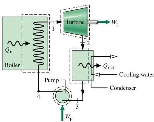
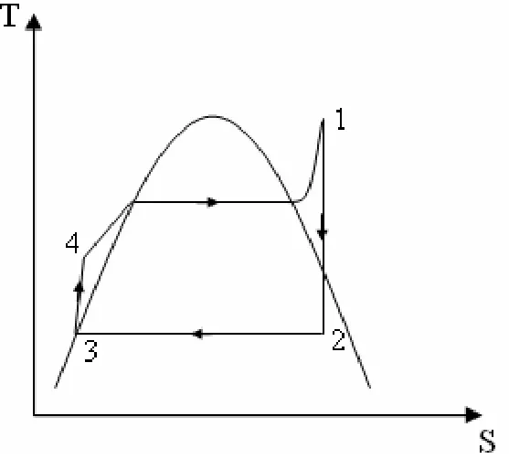
Ideal Rankine cycle is illustrated in the figure.The four processes involved in the complete cycle are different from each other, and each process reqiures a seperate component.Further it may be noted that the working fluid is water which exit in liquid during the part of the cycle and vapur phase in the remaining part of the cycle.

PROCESS IN THE CYCLE:

Process 1-2: Reversible adibatic expansion in the turbine from pressure p1 to p2 to produce the work output.

Process 2-3:Heat transfer from the stem in the condenser.steam is condensed to saturated water at3.

Process 3-4:Reversible adiabatic compression of water in the pump.

Process 4-1: Heat transfer to water at constant pressure in the boiler to produce steam.

IDEAL RANKINE CYCLE:

FORMULAS USED FOR CALCULATIONS:

NET WORK=HEAT SUPPLIED-HEAT REJECTED=QH-QL

HEAT SUPPLIED QH=H1-HF4

HEATREJECTED QL=H2-HF3

NET WORK=TURBINE WORK-PUMP WORK

PUMP WORK WP=V3(P4-P3)

V3=SPECIFIC VPLUME OF WATER AT PUMP INLET

EFFICIENCY OF RANKINE CYCLE=(NET WORK OUTPUT/HEAT SUPPLIED)

EFFICIENCY=(H1-H2)/(H1-HF3)

SPECIFIC STEAM CONSUMPTION=(MASS OF STEAM FLOW/NET WORK OUTPUT)

SSC=(1/(H1-H2))

EXPLANATION OF CODE:

1. Firstly stated the code using close all,clear all,clc commands to clear all the data in command window,work space and plots.
2. Used printf command to print all the process involved the rankine cycle.
3. By using input command, we have taken required inputs from user's side.
4. By calling Xsteam function we have read all the reqired values.
5. Now we have evaluated all the state points by using XSteam function and assigned a variables for storing the data.
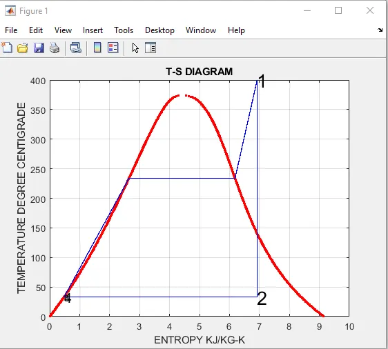
6. By using XSteam we have plotted saturation curve of a T-S daigram and plotted the t-s diagram using state variables.
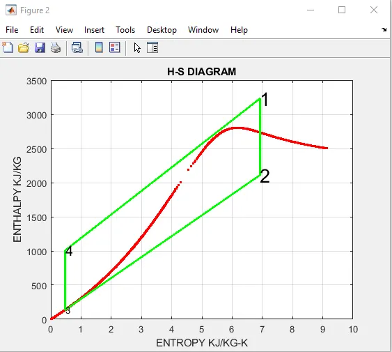
7. By the same procedure we have evaluated h-s daigram.
8. By using some calcuation evaluated all the performance characterstics of rankine cycle.
9. By using fprintf command we have printed all the results obtained.

CODE FOR RANKINE CYCLE SIMULATOR:

%Rankine cycle simulataor as per given conditions
clear all
close all
clc

%title of the result
fprintf('                 RANKINE CYCLE SIMULATOR');
%explaining the process in rankine cycle
fprintf('\n(1-2) ISENTROPIC EXPANSION')
fprintf('\n(2-3) CONSTANT PRESSURE HEAT REJECTION')
fprintf('\n(3-4) ISENTROPIC PUMPING')
fprintf('\n(4-1) CONSTANT PRESSURE HEAT SUPPLY')

%reading inputs from the user and storing in the variables
P1=input('\nENTER THE PRESSURE AT INLET OF THE TURBINE IN BAR:')
T1=input('ENTER THE THEMPERATURE AT INLET OF THE TURBINE IN CENTIGRADE:')
P2=input('ENTER THE PRESSURE AT INLET OF THE CONDENSER AND OUTLET TO TURBINE IN BAR:')

%reading the various parameters required to calculate rankine cycle from
%xsteam data file

%at state1 process(1-2)
H1=XSteam('h_pT',P1,T1); %Enthalpy at state1 
S1=XSteam('s_pT',P1,T1); %Entropy at state1

%at state2 
S2=S1;  %Entropy is equal in isentropic process
SF2=XSteam('sL_p',P2); %entropy at liquid state
SG2=XSteam('sV_p',P2); %entropy at vapour state
HF2=XSteam('hL_p',P2); %enthalpy at liquid state
HG2=XSteam('hV_p',P2); %enthalpy at vapour state
X2=((S2-SF2)/(SG2-SF2));
H2=HF2+(X2*(HG2-HF2)); %enthalpy at state2

%at state3 
P3=P2;                  %pressure is onstant
H3=XSteam('hL_p',P3);   %enthalpy at state3
S3=XSteam('sL_p',P3);   %entropy at state3
V3=XSteam('vL_p',P3);   %volume at state3
T3=XSteam('Tsat_p',P3); %temperature at state3
T2=T3;                  %constant temperature

%at state4
P4=P1;%PRESSURE CONSTANT
S4=S3;%ENTROPY REMAINS CONSTANT AT THIS STAGE 
T4=XSteam('T_ps',P4,S4);%SATURATED TEMPERATURE AT STATE 4
H4=XSteam('hL_p',P4,S4); %ENTHALPY AT STATE4

T5=XSteam('Tsat_p',P1);
S5=XSteam('sL_P',P1);
S6=XSteam('sV_p',P1);
T6=T5;

%input work for pump in KJ/kg
WP=V3*(P4-P3);

%TURBINE WORK
WT=H1-H2; %WORK PRODUCED BY TURBINE

%NET WORK IN RANKINE CYCLE IS
WNET=WT-WP;

%HEAT SUPPLIED IN THE BOILER
QH=H1-H4;

%THERMAL EFFICIENCY OF RANKINE CYCLE 
N_THERM=(WNET/QH)*100;

%back work ratio
BWR=(WP/WT);

%PRINTING THE REULTS
fprintf('--------------------------RESULTS---------------------------------\n')
%printing the parameters at state1
fprintf('AT STATE POINTS1:\n')
fprintf('P1 is : %f bar \n',P1)
fprintf('T1 is : %f deg.centigrade \n',T1)
fprintf('H1 is : %f kj/kgk \n',H1)
fprintf('S1 is : %f kj/kg \n',S1)
%printing the parameters at state2
fprintf('AT STATE POINTS2:\n')
fprintf('P2 is : %f bar \n',P2)
fprintf('T2 is : %f deg.centigrade \n',T2)
fprintf('H2 is : %f kj/kgk \n',H2)
fprintf('S2 is : %f kj/kg \n',S2)
%printing the parameters at state3
fprintf('AT STATE POINTS3:\n')
fprintf('P3 is : %f bar \n',P3)
fprintf('T3 is : %f deg.centigrade \n',T3)
fprintf('H3 is : %f kj/kgk \n',H3)
fprintf('S3 is : %f kj/kg \n',S3)
%printing the parameters at state4
fprintf('AT STATE POINTS4:\n')
fprintf('P4 is : %f bar \n',P4)
fprintf('T4 is : %f deg.centigrade \n',T4)
fprintf('H4 is : %f kj/kgk \n',H4)
fprintf('S4 is : %f kj/kg \n',S4)

%printing the performance parameters of rankine cycle
fprintf('PUMP WORK IS : %f kj/kg\n',WP)       %PUMP WORK
fprintf('TURBINE WORK IS : %f kj/kg\n',WT)    %TURBINE WORK
fprintf('NET WORK IS : %f kj/kg\n',WNET)      %NET WORK 
fprintf('EFFICIENCY IS : %f percentage\n',N_THERM) %EFFICIENCY
fprintf('BACK WORK RATIO IS : %f \n',BWR)       %BACK WORK RATIO


%PLOT T-S and h-s diagram
%plotting t-s diagram
figure(1)
t=linspace(0,400,500);
%plotting saturation curve
for i=1:length(t)
    plot(XSteam('sL_T',t(i)),t(i),'r.')
    plot(XSteam('sV_T',t(i)),t(i),'r.')
    hold on
end
%plotting t-s curve of rankine cycle
plot([S1 S2 S3 S4 S5 S6 S1],[T1 T2 T3 T4 T5 T6 T1],'linewidth',1,'color','b')
grid on
text(S1,T1,'1','fontsize',20)
text(S2,T2,'2','fontsize',20)
text(S3,T3,'3','fontsize',10)
text(S4,T4,'4','fontsize',15)
xlabel('ENTROPY KJ/KG-K')
ylabel('TEMPERATURE DEGREE CENTIGRADE')
title('T-S DIAGRAM')

%PLOTTING H-S DIAGRAM
figure(2)
for i=1:length(t)
    plot(XSteam('sL_T',t(i)),XSteam('hL_T',t(i)),'r.')
    plot(XSteam('sV_T',t(i)),XSteam('hV_T',t(i)),'r.')
    hold on
end
%plotting h-s curve of rankine cycle
plot([S1 S2 S3 S4 S1],[H1 H2 H3 H4 H1],'linewidth',2,'color','g')
grid on
text(S1,H1,'1','fontsize',20)
text(S2,H2,'2','fontsize',20)
text(S3,H3,'3','fontsize',10)
text(S4,H4,'4','fontsize',15)
xlabel('ENTROPY KJ/KG-K')
ylabel('ENTHALPY KJ/KG')
title('H-S DIAGRAM')

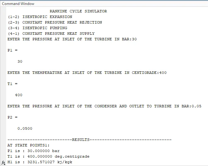
RESULT OBTAINED IN COMMAND WINDOW:

RANKINE CYCLE SIMULATOR
(1-2) ISENTROPIC EXPANSION
(2-3) CONSTANT PRESSURE HEAT REJECTION
(3-4) ISENTROPIC PUMPING
(4-1) CONSTANT PRESSURE HEAT SUPPLY
ENTER THE PRESSURE AT INLET OF THE TURBINE IN BAR:30

P1 =

30

ENTER THE THEMPERATURE AT INLET OF THE TURBINE IN CENTIGRADE:400

T1 =

400

ENTER THE PRESSURE AT INLET OF THE CONDENSER AND OUTLET TO TURBINE IN BAR:0.05

P2 =

0.0500

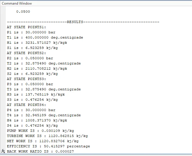
--------------------------RESULTS---------------------------------
AT STATE POINTS1:
P1 is : 30.000000 bar
T1 is : 400.000000 deg.centigrade
H1 is : 3231.571027 kj/kgk
S1 is : 6.923259 kj/kg
AT STATE POINTS2:
P2 is : 0.050000 bar
T2 is : 32.875490 deg.centigrade
H2 is : 2110.708212 kj/kgk
S2 is : 6.923259 kj/kg
AT STATE POINTS3:
P3 is : 0.050000 bar
T3 is : 32.875490 deg.centigrade
H3 is : 137.765119 kj/kgk
S3 is : 0.476254 kj/kg
AT STATE POINTS4:
P4 is : 30.000000 bar
T4 is : 32.945189 deg.centigrade
H4 is : 1008.371370 kj/kgk
S4 is : 0.476254 kj/kg
PUMP WORK IS : 0.030109 kj/kg
TURBINE WORK IS : 1120.862815 kj/kg
NET WORK IS : 1120.832706 kj/kg
EFFICIENCY IS : 50.415297 percentage
BACK WORK RATIO IS : 0.000027

PLOTS FOR T-S AND H-S OF RANKINE CYCLE:

OUT PUT ON THE COMMAND WINDOW:

CONCLUSION:

Rankine cycle simulator is created and plotted t-s and h-s diagram by taking inputs from user and calculated all the rankine cycle parameters and printedon the command window.