Project 2 - Rankine cycle Simulator - MATLAB

OBJECTIVES

• Create a Rankine Cycle Simulator
• Plot T-S and H-S graphs
• Calculate Net work output, Back work ratio and S.S.C

THEORY

• Rankine Cycle

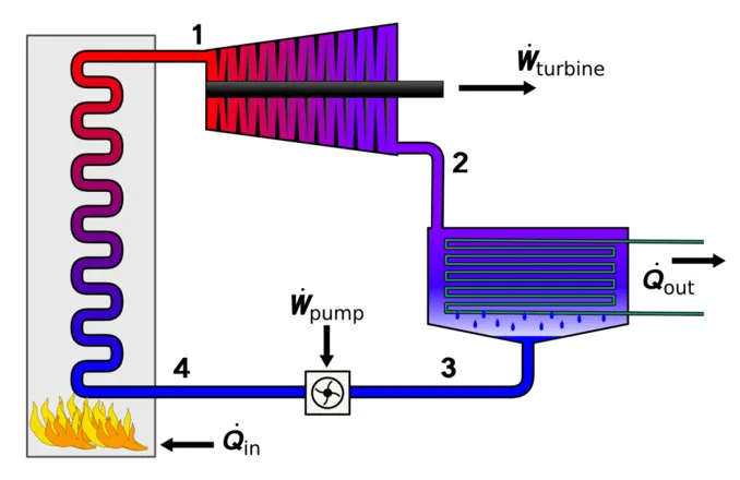
The Rankine cycle is an idealized thermodynamic cycle describing the process by which certain heat engines, such as steam turbines or reciprocating steam engines, allow mechanical work to be extracted from a fluid as it moves between a heat source and heat sink. The Rankine cycle is named after William John Macquorn Rankine, a Scottish polymath professor at Glasgow University.

Heat energy is supplied to the system via a boiler where the working fluid (typically water) is converted to a high pressure gaseous state (steam) in order to turn a turbine. After passing over the turbine the fluid is allowed to condense back into a liquid state as waste heat energy is rejected before being returned to boiler, completing the cycle. Friction losses throughout the system are often neglected for the purpose of simplifying calculations as such losses are usually much less significant than thermodynamic losses, especially in larger systems.

The processes happening in the Rankine cycle are:

Process 1-2 : Isentropic Expansion in Turbine
Process 2-3 : Constant pressure heat rejection
Process 3-4 : Isentropic Compression in Pump
Process 4-1 : Constant pressure heat addition in boiler

Equations used:

• x2 = (s2-sf2)/(sg2-sf2)
• Enthalpy at state point 2, `h_2=hf_2+(x_2(hg_2-hf_2))`
• `gamma=c_p/c_v`
• Temperature at state point 2, `t_4=t_3(p_4/p_3)^((gamma-1)/gamma)`
• Work done by the pump, `W_p=v_3xx(p_4-p_3)xx100`
• Enthalpy at state point 4, `h_4=h_3+W_p`
• Work done by the turbine, `W_t=h_1-h_2`
• Net work output, `W_n=W_t-W_p`
• Heat in, `Q_i=h_1-h_4`
• Heat out, `Q_(out)=h_2-h_3`
• Thermal Efficiency, `eta=W_n/Q_i`
• Back work ratio = `(h_4-h_3)/(h_1-h_2)`
• `SSC=3600/(h_1-h_2)`

MATLAB CODE

% Rankine Cycle Simulator

clear all
close all
clc

% Display
fprintf('        RANKINE CYCLE SIMULATORnn')
fprintf('1-2 Isentropic Expansion in Turbinen')
fprintf('2-3 Constant pressure heat rejectionn')
fprintf('3-4 Isentropic Compression in Pumpn')
fprintf('4-1 Constant pressure heat addition in boilernn')

% User inputs
p1 = input('Turbine inlet pressure, p1 = ');
t1 = input('Turbine inlet temperature, t1 = ');
p2 = input('Condensor inlet pressure, p2 = ');
fprintf('n')

% Calculations

% state 1
s1 = XSteam('s_pT',p1,t1);
h1 = XSteam('h_pT',p1,t1);

% state 2
t2 = XSteam('Tsat_p',p2);
s2 = s1;
sf2 = XSteam('sL_p',p2);
sg2 = XSteam('sV_p',p2);
hf2 = XSteam('hL_p',p2);
hg2 = XSteam('hV_p',p2);
x2 = ((s2-sf2)/(sg2-sf2));
h2 = hf2+(x2*(hg2-hf2));

% state 3
p3 = p2;
t3 = t2;
s3 = XSteam('sL_p',p3);
h3 = XSteam('hL_p',p3);
v3 = XSteam('vL_p',p3);

% state 4
p4 = p1;
s4 = s3;
cp4 = XSteam('Cp_ps',p4,s4);
cv4 = XSteam('Cv_ps',p4,s4);
g4 = cp4/cv4;
o = (g4-1)/g4;
t4 = t3*((p4/p3)^o);


% work done by pump
Wp = v3*(p4-p3)*100;

h4 = h3+Wp;

% state 5
s5 = XSteam('sL_p',p1);
h5 = XSteam('hL_p',p1);
t5 = XSteam('Tsat_p',p1);

% state 6
s6 = XSteam('sV_p',p1);
h6 = XSteam('hV_p',p1);
t6 = t5;


% work done by turbine
Wt = h1-h2;

% net work done
Wnet = Wt-Wp;

% Heat in
Qin = h1-h4;

% Heat out
Qout = h2-h3;

% Thermal efficiency
eff = Wnet/Qin;

% creating array for temperature
T = linspace(0,400,1000);

% entropy and enthalpy values for creating saturation curve
for i=1:length(T)
    sf(i)=XSteam('sL_T',T(i));
    sg(i)=XSteam('sV_T',T(i));
    hf(i)=XSteam('hL_T',T(i));
    hg(i)=XSteam('hV_T',T(i));
end

% T-S diagram
figure(1)
plot(sf,T)
hold on
plot(sg,T)
plot([s1,s2],[t1,t2],'Color','k')
plot([s2,s3],[t2,t3],'Color','k')
plot([s3,s4],[t3,t4],'Color','k')
plot([s4,s5],[t4,t5],'Color','k')
plot([s5,s6],[t5,t6],'Color','k')
plot([s6,s1],[t6,t1],'Color','k')
legend('Saturated Liquid','Saturated Vapour')
axis([0 8 0 450])
xlabel('Entropy(S)')
ylabel('Temperature(T)')
title('T-S diagram')

% H-S diagram
figure(2)
plot(sf,hf,'Color','r')
hold on
plot(sg,hg,'Color','r')
plot([s1,s2],[h1,h2],'Color','k')
plot([s2,s3],[h2,h3],'Color','k')
plot([s3,s4],[h3,h4],'Color','k')
plot([s4,s5],[h4,h5],'Color','k')
plot([s5,s6],[h5,h6],'Color','k')
plot([s6,s1],[h6,h1],'Color','k')
legend('Saturation curve')
axis([0 8 0 450])
xlabel('Entropy(S)')
ylabel('Entahlpy(H)')
title('H-S diagram')

% Back work ratio
Back_work_ratio = (h4-h3)/(h1-h2);

% SSC
SSC = 3600/(h1-h2);

% Displaying Results
fprintf('        RESULTSnn')
fprintf('State point 1:n')
fprintf('P1 = %fn',p1)
fprintf('T1 = %fn',t1)
fprintf('H1 = %fn',h1)
fprintf('S1 = %fnn',s1)

fprintf('State point 2:n')
fprintf('P2 = %fn',p2)
fprintf('T2 = %fn',t2)
fprintf('H2 = %fn',h2)
fprintf('S2 = %fn',s2)
fprintf('X2 = %fnn',x2)

fprintf('State point 3:n')
fprintf('P3 = %fn',p3)
fprintf('T3 = %fn',t3)
fprintf('H3 = %fn',h3)
fprintf('S3 = %fnn',s3)

fprintf('State point 4:n')
fprintf('P4 = %fn',p4)
fprintf('T4 = %fn',t4)
fprintf('H4 = %fn',h4)
fprintf('S4 = %fnn',s4)

fprintf('Work done by Turbine = %fn',Wt)
fprintf('Work done by Pump = %fn',Wp)
fprintf('Net Work done = %fn',Wnet)
fprintf('Thermal Efficiency = %fn',eff)
fprintf('S.S.C = %fn',SSC)

EXPLANATION OF CODES

• fprintf - The fprintf command displays formatted text centered on the icon and can display formatSpec along with the contents of var.
• Line 7 to 12 - Introduction to the problem displaying into the command window.
• Line 15 to 17 - Defining user defined inputs. (p1,t1,p2)
• Line 23 to 66 - Extracting and calculating datas such as pressure,temperature,entropy enthalpy from Xsteam file.
• Line 70 to 82 - Calculating Work done by turbine, Net work done, Heat in, Heat out and Thermal efficiencies.
• Line 85 - creating array for temperature.
• linspace - The linspace function generates linearly spaced vectors.
• Line 88 to 93 - Introducing for loop for finding the entropy and enthalpy values for creating saturation curve.
• Line 96 to 110 - Plotting T-S graph.
• Line 113 to 127 - Plotting H-S graph.
• figure - figure creates figure graphics objects. figure objects are the individual windows on the screen in which MATLAB displays graphical output.
• plot - The plot function in Matlab is used to create a graphical representation of some data.
• hold on - hold on retains plots in the current axes so that new plots added to the axes do not delete existing plots.
• legend - legend creates a legend with descriptive labels for each plotted data series.
• axis - This is used to specify the limits for the current axes.
• xlabel - To label x-axis.
• ylabel - To label y-axis.
• title - Add a title to a plot and return the text object.
• Line 136 to 166 - The results displaying into the command window.

RESULTS

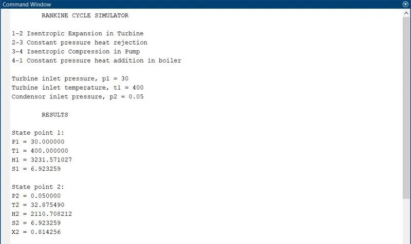
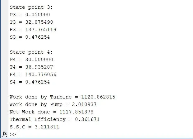
• Screenshot of Command Window

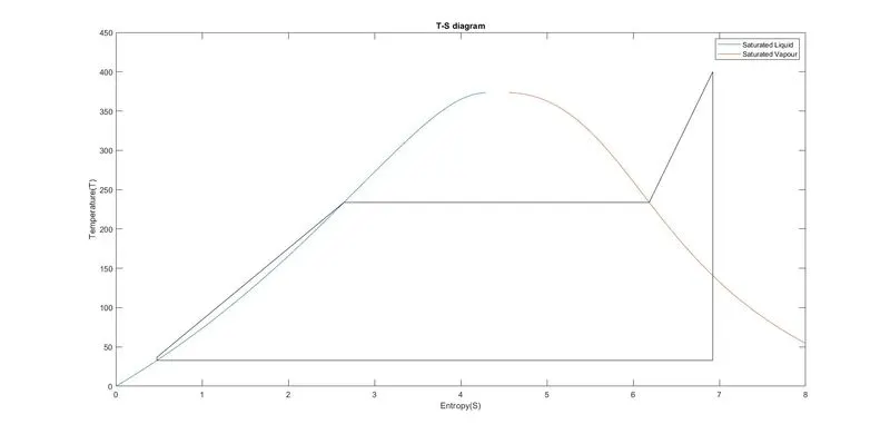
• T-S diagram

• H-S diagram